Boost python with your GPU (numba+CUDA)

Numba + CUDA on Google Colab ¶

By default, Google Colab is not able to run numba + CUDA, because two lilbraries are not found, libdevice and libnvvm.so . So we need to make sure that these libraries are found in the notebook.

First, we look for these libraries on the system. To do that, we simply run the find command, to recursively look for these libraries starting at the root of the filesystem. The exclamation mark escapes the line so that it's executed by the Linux shell, and not by the jupyter notebook.

Then, we add the two libraries to numba environment variables:

And we're done! Now let's get started.

A gentle introduction to ufuncs ¶

Numpy universal functions or ufuncs are functions that operate on a numpy array in an element-by-element fashion. For example, when we take the square of a numpy array, a ufunc computes the square of each element before returning the resulting array:

Most math functions (if not all) are available as ufuncs in numpy. For example, to exponentiate all elements in a numpy array:

Most ufuncs are implemented in compiled C code, so they are already quite fast, and much faster than plain python. For example, let's consider a large array, and let's compute the logarithm of each element, both in plain python and in numpy:

We see that the numpy ufunc is about 50 times faster. Still, in the ufunc, the calculation is not parallelized: the square root is computed sequentially on the CPU for each element in the array.

The GPU, contrary to the CPU, is able to perform a large number of operations simultaneously. In the following, we will see how to create and compile ufuncs for the GPU to perform the calculation on many elements at the same time.

A very simple example : parallel square root calculation on the GPU ¶

Our first ufunc for the GPU will again compute the square root for a large number of points.

We start by building a sample of points ranging from 0 to 10 millions. GPUs are more efficient with numbers that are encoded on a small number of bits. And often, a very high precision is not needed. So we create a sample of float32 numbers (the default being float64 ):

With numba, we can create ufuncs compiled for the CPU using the vectorize decorator. Let's start by doing this:

Creating a ufunc for the GPU is almost as straightforward:

It is important to note that, contrary to the CPU case, the input and return types of the function have to be specified, when compiling for the GPU. In the string:

'float32(float32)'

The first float32 corresponds to the return type, and the second one to the input type. You can think of it as: the returned value is a function of the input value. Also, please note that these types need to be adapted to your data. In the case above, we have created an array of float32 values, so we are fine.

Exercise: Edit the type definition in the vectorize decorator to read float64 , and see what happens when you call the function. Then change it back to float32 .

Now let's see how much we gained. For this, we use the timeit magic command.

The GPU managed to compute the sqrt for 10 million points in 40 ms. Now let's see what we get with numpy, which is compiled for the CPU, and with our CPU ufunc:

Wait! We do not gain anything and the CPU version is actually twice faster!

There is a simple reason for this. When running on the GPU, the following happens under the hood:

• the input data (the array a ) is transferred to the GPU memory;
• the calculation of the square root is done in parallel on the GPU for all elements of a ;
• the resulting array is sent back to the host system.

If the calculation is too simple, there is no use shipping our data to the GPU for fast parallel processing, if we are to wait so long for the data transfers to complete. In other words, most of the time is spent in the data transfers, and the GPU is basically useless.

Let's see what happens with a more involved calculation.

From cartesian to polar coordinates on the GPU ¶

Let's build an array of 1000 points in 2D, described by the cartesian coordinates x and y. We choose to draw the points according to a 2D Gaussian distribution, introducing some correlation between the x and y components:

It's often useful to convert cartesian coordinates into the polar coordinates R and theta , where r is the distance of the point to origin, and where theta is the angle between the x axis and the direction of the point.

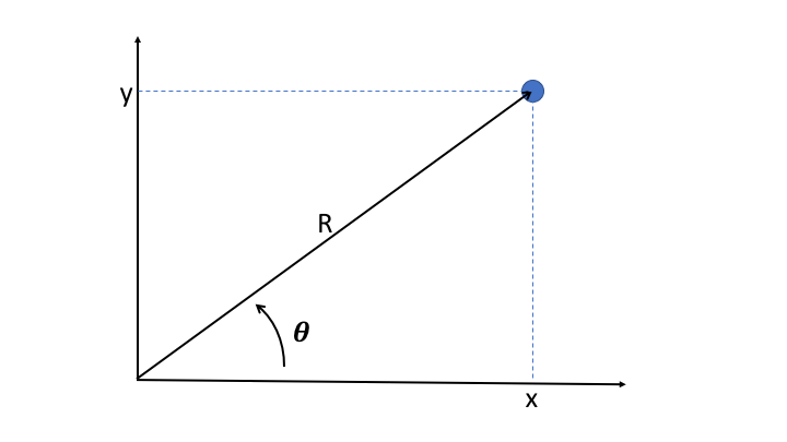
R is easily obtained as the quadratic sum of x and y:

But to get theta, one has to use the arctan2 function. This function is available in numpy, and we can use it to easily get the results (please note that the y coordinate has to be provided as the first argument)

Because of the correlation between x and y, we see two peaks at $\pi/4$ and $-3\pi/4$.

Now let's try and perform the same calculation on the GPU. This time, we have two input values, and we define the function signature accordingly.

As before with np.arctan2 , we need to slice our points array to provide first the array of y coordinates, and then the array of x coordinates:

Hmm this doesn't work. As the exception says, it is because points[:,1] contain values that are not contiguous in memory, and same for points[:,2] . So we do as instructed and convert these slices into contiguous arrays:

And now it works!

As a general rule, one should remember that CUDA operates on data buffers that are contiguous in memory, like a C array, or a numpy array before any slicing.

Now let's be a bit more ambitious, and compute theta for 10 million points:

And finally, let's quantify how much time we gain by running on the GPU:

Nice! this time we gain almost a factor 10 on the GPU with respect to the numpy version, which is compiled for the CPU. And this comes on top of a factor 20 gain with respect to plain python.

Remember: To use the GPU efficiently, you need to give it enough data to process, and complicated tasks.

Generalized ufuncs on the GPU ¶

In regular ufuncs, the calculation is done on each element of the input array, and returns a scalar.

In generalized ufuncs (gufuncs), however, the calculation can deal with a sub-array of the input array, and return an array of different dimensions.

Ok, I know that sometimes what I write does not make sense... But at least I realize it! So let's have a look at a few examples, things are going to become much clearer.

Generalized ufuncs : from cartesian to polar coordinates ¶

Remember how we computed the polar angle for our 2D points above? It would have been nice to get both rho and theta from this calculation, to get a real conversion from cartesian to polar coordinates. This kind of thing is not possible with regular ufuncs (or maybe I just don't know how to do it). But with gufuncs, it's easy:

There are two imporant differences between guvectorize and vectorize .

For guvectorize :

• one needs to provide the signature of the array operation . The signature of the array operation should not to confused with the signature of the compiled function that is provided as a first argument. In the example above, (i)->(i) means that a 1D array is taken in input, and that a 1D array with the same size is provided in the output. The 1D array corresponds to the last dimension or innermost dimension of the input array. For example, our points array is of shape (10000000,2) so the last dimension is of size 2.
• the result is taken in input and modified in place . In the code above, the resulting polar coordinates R and theta are stored in the out array while vec , the input array, contains the cartesian coordinates x and y .

Let's do the conversion between cartesian and polar coordinates:

Generalized ufunc: Average ¶

To understand better how gufuncs work, let's make one that computes the average of the values on each line of a 2D array:

To test our gufunc, we create a 2D array:

Device functions ¶

So far, we have run a single function, either a ufunc or a gufunc, on the GPU, but we are not forced to put all of our code in a single function.

Indeed, it is also possible to compile helper functions for the GPU. These functions, called device functions , can then be used on the GPU to make the code cleaner and more modular.

As an example, let's take again the gufunc defined just above, that computes the average of the values of each line of a 2D array.

We define a device function to add the using the numba.cuda.jit decorator, to sum up the elements of a 1D array. Then, we modify the gpu_average gufunc to make use of the add device function. And finally, we create another gufunc to sum up the elements of on each line of a 2D array:

The device function allows us to avoid code duplication.

Obviously, it is a bit artifial to use a device function in such an easy case. But when implementing complex algorithms, these functions can prove very useful. Indeed, just like on the CPU, the general principles of programming apply: functions should be simple and to the point, and code duplication should be avoided.

Memory management with device arrays ¶

As we have seen in the first ufunc example given in this article (parallel square root calculation), the GPU does not always provide a gain in performance.

Indeed, before using the raw computing power of the GPU, we need to ship the data to the device. And afterwards, we need to get the results back.

A good way to improve performance is to minimize data transfers between the host system and the GPU, and this can be done with device arrays.

To illustrate this, we will use an example provided by nvidia in its DLI course. Let's assume we want to implement a neural network for image processing from scratch. A hidden layer in the network might have to do the following:

• normalize greyscale values in the image
• weigh them
• apply an activation function

Each of these three tasks can be done in parallel on the GPU.

But first, let's see how to do that on the CPU with plain numpy. For simplicity, we will generate the greyscale values and the weights randomly.

Now, we implement a parallel version of this algorithm for the GPU, as we have seen above.

Please note that the code in these ufuncs operates on scalar values, so we replaced the numpy ufuncs like np.exp by their math equivalent (the division by 255 and the multiplication between the values and the weights were also numpy ufuncs, though hidden a bit).

And we check the performance:

That's already quite nice, we gained more than a factor of two!

But we realize that we spend time transferring data back and forth between the host and the GPU for nothing:

1. transfer greyscales to the GPU
2. transfer normalized to the host, and then back to the GPU, together with weights
3. transfer weighted to the host, and then back to the GPU
4. transfer activated to the host

Actually, we only need to:

1. transfer greyscales and weights to the GPU
2. retrieve activated

So let's do that:

We gain a factor of two by eliminating unnecessary data transfers!

Another important thing to know is that we can also take full control on the transfers to and from the GPU like this:

Now that everything we need is on the GPU, we do the calculation:

You might be thinking that this factor 5 gain is artificial, because we did not include the necessary transfer times for the input and output data. That's right! Still, this illustrates how you can take full control of your data transfers, which might prove useful on more complex processing workflows.

For instance, if we wanted to re-use any of the device arrays defined above, we could do it now, as they are still residing on the GPU as I'm writing this!

Finally, here is how to retrieve the results: