Image Recognition with Transfer Learning (98.5%)

Use transfer learning to easily classify dog and cat pictures with a 98.5% accuracy.

Transfer learning between robots
Transfer learning.

Outline

In this article, you will learn how to use transfer learning for powerful image recognition, with keras, TensorFlow, and state-of-the-art pre-trained neural networks: VGG16, VGG19, and ResNet50.

In the process, you will understand what is transfer learning, and how to do a few technical things:

  • add layers to an existing pre-trained neural network to adapt it to your needs.
  • save a keras model so that you can re-use it later on, without having to retrain.
  • evaluate the model performance and have a look at misidentified pictures.

*Please keep in mind that this post does not provide a comparison of performance between the three models. That would be quite difficult to do in a proper and fair way.*

But first ...

What is transfer learning?

In the previous article, Image Recognition: Dogs vs Cats! , we have seen how to build a simple convolutional network from scratch to classify dog and cat pictures with a 92% accuracy.

Modern convolutional neural networks such as VGG, ResNet, or Inception, would be able to perform this task with an accuracy over 99%. But these models are deep and complex. So they are hard to train, and a very large number of images are necessary to train these networks without overfitting .

In fact, these models are now trained on the ImageNet dataset, which features over 14 million images sorted in 1000 categories. Compared to that, our dogs and cats dataset, with its 25 000 images, is ridiculously small. And we have seen in the previous article that even with our simple network, we are forced to use strong data augmentation to limit overfitting. So training a complex model on this dataset is out of question.

So how can we improve the classification performance on our small dataset if there is no way to train a complex model on this dataset?

The solution is transfer learning, and it's technically very easy to implement as we will see!

Here's the idea.

First, consider the architecture of the VGG16 convolutional network, shown below.

Fig. A1. The standard VGG-16 network architecture as proposed in [32]. Note that only layers “conv1” to “fc7” are used in the feature extractor.
VGG16 architecture (illustration from Max Ferguson)

In the first part of the network, we see five convolutional blocks (conv1 to 5), which consist in stacked convolutional layers followed by a max pooling layer (you can find an explanation about these layers here ). So we'll call this part the convolutional part.

This part produces a tensor with 7x7x512 values for each image. The first two dimensions, (7,7), are aligned with the dimensions of the original image, and we can think of this as a very coarse version of the image, with only 7x7=49 large pixels. But for each pixel, instead of having 3 color channels, we have 512 features that describe what the network is seeing in this pixel (and also around it).

This tensor therefore contains 7x7x512 = 25 088 numbers that are the features extracted by the network for the image.

But what exactly are these "features"?

In my post about Real Time Human Detection with OpenCV we have used a clever (and fairly complicated) algorithm, the Histograms of Oriented Gradients (HOG), to extract the image features (basically the edges in the image). These features are then interpreted by a Support Vector Machine (SVM) to decide whether there is a human in the detection window or not.

Here, and generally speaking in deep learning, we instead let the network discover the features by itself during the training! No need to design and code a complicated feature extraction algorithm, we just give the network a structure with enough flexibility, and we train it by examples.
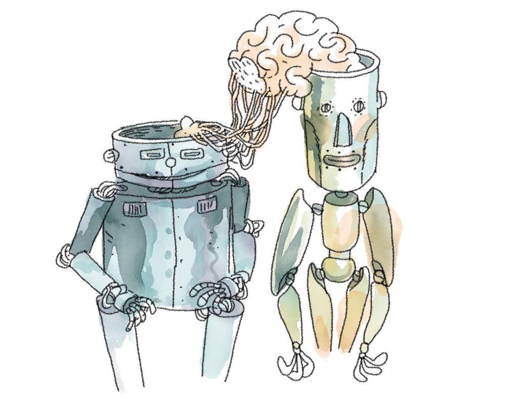
Think of a baby.

A baby starts to see
Second day, can already see.

I don't know much about the human brain nor human vision, and have only limited experience with babies! (got two.) Anyway here is what I think. Take it as an analogy, maybe it's right, maybe it's wrong, but I find it interesting.

During the very first hours of its life, the baby has to learn how to see. And by that I mean to make sense of the overwhelming signal streams that come from her eyes. I suspect that at first, the baby learns how to see lines, by connecting the information from neighbouring retina rods and cones. Then, she starts seeing shapes, and recognizing objects. This is some kind of an unsupervised learning process: you just need to move your eyes to see that things are connected, no need to be shown examples. And much, much later, the baby will be able to use supervised learning: cat! she says. No, this is a tiger.

VGG16 was trained on the large ImageNet dataset and is already able to see.

But it has also been trained to classify the images in the 1000 categories of ImageNet.

The classification occurs in the second part of the model, which takes the image features in input and picks a category. This classifier part contains:

  • two hidden fully connected (or dense) layers, each with 4096 neurons.
  • a dense layer with 1000 neurons, one for each of the ImageNet categories. The softmax activation function is used for these neurons, so that the 1000 values they spit out sum up to unity, and can be considered as probabilities.

What we're going to do, for VGG16 and the other pre-trained models, is to download the model with the weights resulting from the training on ImageNet. Then, we will replace the classifier part by our own simple classifier, adapted to our problem. For instance, this classifier will have only two output neurons in the last layer, one for dog and one for cat. Finally, we will freeze all the layers of the convolutional part, so that we only have to train the parameters of our classifier on our small dataset.

So let's see how to do this technically with keras.

Running this tutorial

To run this tutorial, you will need:

  • a Linux or Windows PC with a GPU.
  • specific python packages for deep learning (Keras, TensorFlow) and to analyze the results (numpy, matplotlib)
  • the dogs and cats dataset.

If you want to set this up, please refer to the instructions in my first post Image Recognition: Dogs vs Cats! (92%) .

When, you're done, specify in the cell below the location of the dataset directory, which the one that contains the dogs and cats subdirectories. Then, execute the cell to import the required packages.

In [1]:
# define and move to dataset directory
datasetdir = '/data2/cbernet/maldives/dogs_vs_cats'
import os
os.chdir(datasetdir)

# import the needed packages
import matplotlib.pyplot as plt
import matplotlib.image as img
import tensorflow.keras as keras
import numpy as np

A couple tools

We're going to start by defining two functions that we will need later.

The first function, generators , returns two image iterators that we will use to produce batches of images for the training and the validation of our neural networks.

In [2]:
from tensorflow.keras.preprocessing.image import ImageDataGenerator

batch_size = 30

def generators(shape, preprocessing): 
    '''Create the training and validation datasets for 
    a given image shape.
    '''
    imgdatagen = ImageDataGenerator(
        preprocessing_function = preprocessing,
        horizontal_flip = True, 
        validation_split = 0.1,
    )

    height, width = shape

    train_dataset = imgdatagen.flow_from_directory(
        os.getcwd(),
        target_size = (height, width), 
        classes = ('dogs','cats'),
        batch_size = batch_size,
        subset = 'training', 
    )

    val_dataset = imgdatagen.flow_from_directory(
        os.getcwd(),
        target_size = (height, width), 
        classes = ('dogs','cats'),
        batch_size = batch_size,
        subset = 'validation'
    )
    return train_dataset, val_dataset
    

The functions has two parameters, shape and preprocessing , which depend on the pre-trained model in use.

The iterators load the dog and cat images from the disk and convert these images to arrays with the given shape . If the shape is wrong, the images will not be adapted to the model, and the code will crash. So we'll have to be careful to choose the correct shape for each pre-trained model we're going to use. VGG16, VGG19, and ResNet50 all take images of shape (224,224,3), so with three color channels in 224x224 pixels. But InceptionV3, for example, would take images of shape (299,299,3).

The iterators are created by a keras ImageDataGenerator that does the following:

  • it has a 50% chance to flip left and right in the image. This provides basic data augmentation without much cost in terms of computing. Indeed, the flipping is easily carried out under the hood by numpy in a very efficient way.
  • then it applies the preprocessing function to the image. This function should be adapted to the pre-trained model in use, and is passed to the generators function as an argument. Indeed, in python, a function is an object, that can happily be passed around to other functions).
  • it keeps 90% of the images for training, reserving 10% of the images for validation. Since we have about 25 000 images in our dataset in total, this leaves 2500 images for a rather accurate validation (more on this later).

The second function will be used to plot the accuracy and loss as a function of the epoch, so that we can see how the training worked. To get a feeling for overfitting, these quantities will be plotted for both the training and validation datasets:

In [3]:
def plot_history(history, yrange):
    '''Plot loss and accuracy as a function of the epoch,
    for the training and validation datasets.
    '''
    acc = history.history['acc']
    val_acc = history.history['val_acc']
    loss = history.history['loss']
    val_loss = history.history['val_loss']

    # Get number of epochs
    epochs = range(len(acc))

    # Plot training and validation accuracy per epoch
    plt.plot(epochs, acc)
    plt.plot(epochs, val_acc)
    plt.title('Training and validation accuracy')
    plt.ylim(yrange)
    
    # Plot training and validation loss per epoch
    plt.figure()

    plt.plot(epochs, loss)
    plt.plot(epochs, val_loss)
    plt.title('Training and validation loss')
    
    plt.show()

We're now ready to get started with our first pre-trained model.

VGG16

The first VGG models were created by Karen Simonyan and Andrew Zisserman, and first presented in the paper Very Deep Convolutional Networks for Large-Scale Image Recognition in 2015. VGG16 has 16 layers with weights, and VGG99 has 19 layers with weights.

At the time, VGG models really came as a breakthrough, for a number of reasons. First, the authors were able to outperform the competition by a large amount on the Image Net Large-Scale Visual Recognition Challenge (ILSVRC). Then, they showed that, with transfer learning, their models generalize well to other image recognition tasks on smaller datasets (see Appendix B in the paper), achieving state-of-the art performance on these datasets as well. Finally, they made their best-performing networks available to the public for further research and practical applications.

Surprisingly enough, the VGG architecture is quite straightforward and very similar to the original convolutional networks. The main idea behind VGG was to make the network deeper by stacking more convolutional layers. And this was made possible by restricting the size of the convolutional windows to only 3x3 pixels.

Feature extraction with VGG16

So let's have a look at the VGG16 architecture. For this, we create an instance of the VGG16 model with keras, and we print the summary:

In [4]:
vgg16 = keras.applications.vgg16
vgg = vgg16.VGG16(weights='imagenet')
vgg.summary()
_________________________________________________________________
Layer (type)                 Output Shape              Param #   
=================================================================
input_1 (InputLayer)         (None, 224, 224, 3)       0         
_________________________________________________________________
block1_conv1 (Conv2D)        (None, 224, 224, 64)      1792      
_________________________________________________________________
block1_conv2 (Conv2D)        (None, 224, 224, 64)      36928     
_________________________________________________________________
block1_pool (MaxPooling2D)   (None, 112, 112, 64)      0         
_________________________________________________________________
block2_conv1 (Conv2D)        (None, 112, 112, 128)     73856     
_________________________________________________________________
block2_conv2 (Conv2D)        (None, 112, 112, 128)     147584    
_________________________________________________________________
block2_pool (MaxPooling2D)   (None, 56, 56, 128)       0         
_________________________________________________________________
block3_conv1 (Conv2D)        (None, 56, 56, 256)       295168    
_________________________________________________________________
block3_conv2 (Conv2D)        (None, 56, 56, 256)       590080    
_________________________________________________________________
block3_conv3 (Conv2D)        (None, 56, 56, 256)       590080    
_________________________________________________________________
block3_pool (MaxPooling2D)   (None, 28, 28, 256)       0         
_________________________________________________________________
block4_conv1 (Conv2D)        (None, 28, 28, 512)       1180160   
_________________________________________________________________
block4_conv2 (Conv2D)        (None, 28, 28, 512)       2359808   
_________________________________________________________________
block4_conv3 (Conv2D)        (None, 28, 28, 512)       2359808   
_________________________________________________________________
block4_pool (MaxPooling2D)   (None, 14, 14, 512)       0         
_________________________________________________________________
block5_conv1 (Conv2D)        (None, 14, 14, 512)       2359808   
_________________________________________________________________
block5_conv2 (Conv2D)        (None, 14, 14, 512)       2359808   
_________________________________________________________________
block5_conv3 (Conv2D)        (None, 14, 14, 512)       2359808   
_________________________________________________________________
block5_pool (MaxPooling2D)   (None, 7, 7, 512)         0         
_________________________________________________________________
flatten (Flatten)            (None, 25088)             0         
_________________________________________________________________
fc1 (Dense)                  (None, 4096)              102764544 
_________________________________________________________________
fc2 (Dense)                  (None, 4096)              16781312  
_________________________________________________________________
predictions (Dense)          (None, 1000)              4097000   
=================================================================
Total params: 138,357,544
Trainable params: 138,357,544
Non-trainable params: 0
_________________________________________________________________

We clearly see the convolutional part and the classifier part. Between the two, a Flatten layer converts the feature tensor of shape (7,7,512) to a 1D array with 7x7x512 = 25088 values, that can be sent as input to the first Dense layer of the classifier.

The classifier is adapted to the 1000 categories of ImageNet. Our task, however, is to classify dog and cat pictures, so we have only two categories.

What can we do? With keras, it's easy to import only the convolutional part of VGG16, by setting the include_top parameter to False :

In [5]:
vgg16 = keras.applications.vgg16
conv_model = vgg16.VGG16(weights='imagenet', include_top=False)
conv_model.summary()
_________________________________________________________________
Layer (type)                 Output Shape              Param #   
=================================================================
input_2 (InputLayer)         (None, None, None, 3)     0         
_________________________________________________________________
block1_conv1 (Conv2D)        (None, None, None, 64)    1792      
_________________________________________________________________
block1_conv2 (Conv2D)        (None, None, None, 64)    36928     
_________________________________________________________________
block1_pool (MaxPooling2D)   (None, None, None, 64)    0         
_________________________________________________________________
block2_conv1 (Conv2D)        (None, None, None, 128)   73856     
_________________________________________________________________
block2_conv2 (Conv2D)        (None, None, None, 128)   147584    
_________________________________________________________________
block2_pool (MaxPooling2D)   (None, None, None, 128)   0         
_________________________________________________________________
block3_conv1 (Conv2D)        (None, None, None, 256)   295168    
_________________________________________________________________
block3_conv2 (Conv2D)        (None, None, None, 256)   590080    
_________________________________________________________________
block3_conv3 (Conv2D)        (None, None, None, 256)   590080    
_________________________________________________________________
block3_pool (MaxPooling2D)   (None, None, None, 256)   0         
_________________________________________________________________
block4_conv1 (Conv2D)        (None, None, None, 512)   1180160   
_________________________________________________________________
block4_conv2 (Conv2D)        (None, None, None, 512)   2359808   
_________________________________________________________________
block4_conv3 (Conv2D)        (None, None, None, 512)   2359808   
_________________________________________________________________
block4_pool (MaxPooling2D)   (None, None, None, 512)   0         
_________________________________________________________________
block5_conv1 (Conv2D)        (None, None, None, 512)   2359808   
_________________________________________________________________
block5_conv2 (Conv2D)        (None, None, None, 512)   2359808   
_________________________________________________________________
block5_conv3 (Conv2D)        (None, None, None, 512)   2359808   
_________________________________________________________________
block5_pool (MaxPooling2D)   (None, None, None, 512)   0         
=================================================================
Total params: 14,714,688
Trainable params: 14,714,688
Non-trainable params: 0
_________________________________________________________________

You can check in the summary that the classifier has indeed been removed.

The convolutional model can already be used to extract the features for a given image:

In [6]:
from keras.preprocessing import image

img_path = 'dogs/dog.1.jpg'

# loading the image: 
img = image.load_img(img_path, target_size=(224, 224))
# turn it into a numpy array
x = image.img_to_array(img)
print(np.min(x), np.max(x))
print(x.shape)
# expand the shape of the array, 
# a new axis is added at the beginning:
xs = np.expand_dims(x, axis=0)
print(xs.shape)
# preprocess input array for VGG16
xs = vgg16.preprocess_input(xs)
# evaluate the model to extract the features
features = conv_model.predict(xs)
print(features.shape)
Using TensorFlow backend.
0.0 255.0
(224, 224, 3)
(1, 224, 224, 3)
(1, 7, 7, 512)

Let's take a closer look at this code.

The first important thing to note is that the predict method of our model is designed to work on several images. These images are supposed to be stored in a numpy array with shape (n,224,224,3) , where n is the number of images to be processed. So first, we have loaded an image, and converted it to a numpy array of shape (224,224,3) . To match the signature of the predict method, we then created an array of shape (1,224,224,3) with np.expand_dims .

The other important point is that VGG16 has been trained on pre-processed images. Quoting the VGG paper:

"The only processing we do is subtracting the mean RGB value, computed on the training set, from each pixel"

To reach maximum performance, it is important to apply the exact same preprocessing before evaluating the network. Keras advocates the use of vgg16.preprocess_inputs for this, so that's what we're going to do.

You may print the feature tensor if you wish, but that's not going to tell you much. This is really just a (big) bunch of numbers. To make sense of these numbers, we need to create our own classifier.

One possibility could be to store the features in data arrays for each image. Then, we could train a small neural network on these arrays. This approach would be perfectly viable. However, that's not what we're going to do. Instead, we will extend VGG16 with our own classifier. This solution is easier to implement and is also more flexible.

Custom classification with VGG16

In the Keras documentation for VGG16 , and also in the original paper, we see that the input of VGG16 should be images with 224x224 pixels. And we also know that the images have to be preprocessed in the correct way for this model. So we create training and validation iterators to produce such images, with the function we have defined at the beginning of this post:

In [7]:
train_dataset, val_dataset = generators((224,224), preprocessing=vgg16.preprocess_input)
Found 22481 images belonging to 2 classes.
Found 2496 images belonging to 2 classes.

As you can see, I don't have all 25 000 images of the dogs and cats dataset. This is because I have cleaned up the dataset to remove a few really bad examples, as explained in Image Recognition: Dogs vs Cats . If you haven't done that, don't worry, this tutorial will work just fine.

We create the convolutional part again, as we need to specify the input_shape this time to be able to create the full model:

In [8]:
conv_model = vgg16.VGG16(weights='imagenet', include_top=False, input_shape=(224,224,3))

If you don't specify input_shape , the dimensions of the network remain undefined, and you end up with the following error message when you try to create the first Dense layer of the classifier below.

ValueError: The last dimension of the inputs to `Dense` should be defined. Found `None`.

Then we plug the output of the convolutional part into a classifier:

In [9]:
# flatten the output of the convolutional part: 
x = keras.layers.Flatten()(conv_model.output)
# three hidden layers
x = keras.layers.Dense(100, activation='relu')(x)
# final softmax layer with two categories (dog and cat)
predictions = keras.layers.Dense(2, activation='softmax')(x)

# creating the full model:
full_model = keras.models.Model(inputs=conv_model.input, outputs=predictions)
full_model.summary()
_________________________________________________________________
Layer (type)                 Output Shape              Param #   
=================================================================
input_3 (InputLayer)         (None, 224, 224, 3)       0         
_________________________________________________________________
block1_conv1 (Conv2D)        (None, 224, 224, 64)      1792      
_________________________________________________________________
block1_conv2 (Conv2D)        (None, 224, 224, 64)      36928     
_________________________________________________________________
block1_pool (MaxPooling2D)   (None, 112, 112, 64)      0         
_________________________________________________________________
block2_conv1 (Conv2D)        (None, 112, 112, 128)     73856     
_________________________________________________________________
block2_conv2 (Conv2D)        (None, 112, 112, 128)     147584    
_________________________________________________________________
block2_pool (MaxPooling2D)   (None, 56, 56, 128)       0         
_________________________________________________________________
block3_conv1 (Conv2D)        (None, 56, 56, 256)       295168    
_________________________________________________________________
block3_conv2 (Conv2D)        (None, 56, 56, 256)       590080    
_________________________________________________________________
block3_conv3 (Conv2D)        (None, 56, 56, 256)       590080    
_________________________________________________________________
block3_pool (MaxPooling2D)   (None, 28, 28, 256)       0         
_________________________________________________________________
block4_conv1 (Conv2D)        (None, 28, 28, 512)       1180160   
_________________________________________________________________
block4_conv2 (Conv2D)        (None, 28, 28, 512)       2359808   
_________________________________________________________________
block4_conv3 (Conv2D)        (None, 28, 28, 512)       2359808   
_________________________________________________________________
block4_pool (MaxPooling2D)   (None, 14, 14, 512)       0         
_________________________________________________________________
block5_conv1 (Conv2D)        (None, 14, 14, 512)       2359808   
_________________________________________________________________
block5_conv2 (Conv2D)        (None, 14, 14, 512)       2359808   
_________________________________________________________________
block5_conv3 (Conv2D)        (None, 14, 14, 512)       2359808   
_________________________________________________________________
block5_pool (MaxPooling2D)   (None, 7, 7, 512)         0         
_________________________________________________________________
flatten (Flatten)            (None, 25088)             0         
_________________________________________________________________
dense (Dense)                (None, 100)               2508900   
_________________________________________________________________
dense_1 (Dense)              (None, 100)               10100     
_________________________________________________________________
dense_2 (Dense)              (None, 100)               10100     
_________________________________________________________________
dense_3 (Dense)              (None, 2)                 202       
=================================================================
Total params: 17,243,990
Trainable params: 17,243,990
Non-trainable params: 0
_________________________________________________________________

We lock all the layers of the convolutional part:

In [10]:
for layer in conv_model.layers:
    layer.trainable = False

And we check that the only layers that will be trained are the ones of the dense classifier:

In [11]:
full_model.summary()
_________________________________________________________________
Layer (type)                 Output Shape              Param #   
=================================================================
input_3 (InputLayer)         (None, 224, 224, 3)       0         
_________________________________________________________________
block1_conv1 (Conv2D)        (None, 224, 224, 64)      1792      
_________________________________________________________________
block1_conv2 (Conv2D)        (None, 224, 224, 64)      36928     
_________________________________________________________________
block1_pool (MaxPooling2D)   (None, 112, 112, 64)      0         
_________________________________________________________________
block2_conv1 (Conv2D)        (None, 112, 112, 128)     73856     
_________________________________________________________________
block2_conv2 (Conv2D)        (None, 112, 112, 128)     147584    
_________________________________________________________________
block2_pool (MaxPooling2D)   (None, 56, 56, 128)       0         
_________________________________________________________________
block3_conv1 (Conv2D)        (None, 56, 56, 256)       295168    
_________________________________________________________________
block3_conv2 (Conv2D)        (None, 56, 56, 256)       590080    
_________________________________________________________________
block3_conv3 (Conv2D)        (None, 56, 56, 256)       590080    
_________________________________________________________________
block3_pool (MaxPooling2D)   (None, 28, 28, 256)       0         
_________________________________________________________________
block4_conv1 (Conv2D)        (None, 28, 28, 512)       1180160   
_________________________________________________________________
block4_conv2 (Conv2D)        (None, 28, 28, 512)       2359808   
_________________________________________________________________
block4_conv3 (Conv2D)        (None, 28, 28, 512)       2359808   
_________________________________________________________________
block4_pool (MaxPooling2D)   (None, 14, 14, 512)       0         
_________________________________________________________________
block5_conv1 (Conv2D)        (None, 14, 14, 512)       2359808   
_________________________________________________________________
block5_conv2 (Conv2D)        (None, 14, 14, 512)       2359808   
_________________________________________________________________
block5_conv3 (Conv2D)        (None, 14, 14, 512)       2359808   
_________________________________________________________________
block5_pool (MaxPooling2D)   (None, 7, 7, 512)         0         
_________________________________________________________________
flatten (Flatten)            (None, 25088)             0         
_________________________________________________________________
dense (Dense)                (None, 100)               2508900   
_________________________________________________________________
dense_1 (Dense)              (None, 100)               10100     
_________________________________________________________________
dense_2 (Dense)              (None, 100)               10100     
_________________________________________________________________
dense_3 (Dense)              (None, 2)                 202       
=================================================================
Total params: 17,243,990
Trainable params: 2,529,302
Non-trainable params: 14,714,688
_________________________________________________________________

Indeed, we see that the number of trainable parameters is the total number of parameters in the last 4 dense layers:

In [12]:
2508900+10100*2+202
Out[12]:
2529302

We can now compile and train the model:

In [13]:
full_model.compile(loss='binary_crossentropy',
                  optimizer=keras.optimizers.Adamax(lr=0.001),
                  metrics=['acc'])
history = full_model.fit_generator(
    train_dataset, 
    validation_data = val_dataset,
    workers=10,
    epochs=5,
)
Epoch 1/5
750/750 [==============================] - 73s 97ms/step - loss: 0.1518 - acc: 0.9685 - val_loss: 0.0731 - val_acc: 0.9760
Epoch 2/5
750/750 [==============================] - 71s 94ms/step - loss: 0.0409 - acc: 0.9876 - val_loss: 0.0627 - val_acc: 0.9812
Epoch 3/5
750/750 [==============================] - 72s 96ms/step - loss: 0.0329 - acc: 0.9913 - val_loss: 0.0642 - val_acc: 0.9820
Epoch 4/5
750/750 [==============================] - 71s 94ms/step - loss: 0.0232 - acc: 0.9932 - val_loss: 0.0743 - val_acc: 0.9784
Epoch 5/5
750/750 [==============================] - 72s 96ms/step - loss: 0.0182 - acc: 0.9950 - val_loss: 0.0749 - val_acc: 0.9800
In [14]:
plot_history(history, yrange=(0.9,1))

We see that the model is very fast to train, as we just need to train the classifier part. One epoch is actually enough to reach a validation accuracy of about 98%, much higher than the 92% we got when we trained a simple convolutional network from scratch on our own in Image Recognition: Dogs vs Cats! .

After that, the accuracy plateaus. Overfitting is moderate and is limiting performance. We could probably work on overfitting by simplifying the classifier, or by adding a dropout layer just before the classifier. But this is out of scope for this post.

A brief digression about statistical uncertainty

Note that value of the accuracy should not be taken too seriously. The validation accuracy depends on the specific validation sample that has been chosen by the generator, and this number is affected by statistical uncertainty. Roughly speaking, we have 2500 images in the validation dataset. An inaccuracy of 2% means that we misclassify 50 images.

Since this number is fairly small, it is affected by fairly large statistical uncertainty. And we can estimate the relative uncertainty on this number as $1/\sqrt{50} \sim 15\%$. The relative uncertainty on the inaccuracy is also of the order of 15%. So for a 2% inaccuracy, we have an absolute uncertainty of 2 x 0.15 = 0.3%.

Therefore, when we talk about a 98% accuracy, you should remember that the true accuracy should within $98 \pm 0.3\%$.

We could use a larger validation dataset to reduce the uncertainty, but this would leave less images for the training of our neural networks.

VGG19

VGG19 is the most recent version of the VGG models and is very similar to VGG16. If you compare the model summary below to the one of VGG16, you will see that the architecture is the same, and is still based on five convolutional blocks.

However, the depth of the network has been further increased by adding a convolutional layer in the last three blocks.

The input is still an RGB image of shape (224,224,3), and the output a feature tensor of shape (7,7,512). Keras provides a specific preprocessing function for VGG19, but if you look at the code, you'll see that it's the exact same function as for VGG 16. So we don't need to redefine our dataset iterators.

Now let's build and check the full model:

In [15]:
vgg19 = keras.applications.vgg19
conv_model = vgg19.VGG19(weights='imagenet', include_top=False, input_shape=(224,224,3))
for layer in conv_model.layers: 
    layer.trainable = False
x = keras.layers.Flatten()(conv_model.output)
x = keras.layers.Dense(100, activation='relu')(x)
predictions = keras.layers.Dense(2, activation='softmax')(x)
full_model = keras.models.Model(inputs=conv_model.input, outputs=predictions)
full_model.summary()
_________________________________________________________________
Layer (type)                 Output Shape              Param #   
=================================================================
input_4 (InputLayer)         (None, 224, 224, 3)       0         
_________________________________________________________________
block1_conv1 (Conv2D)        (None, 224, 224, 64)      1792      
_________________________________________________________________
block1_conv2 (Conv2D)        (None, 224, 224, 64)      36928     
_________________________________________________________________
block1_pool (MaxPooling2D)   (None, 112, 112, 64)      0         
_________________________________________________________________
block2_conv1 (Conv2D)        (None, 112, 112, 128)     73856     
_________________________________________________________________
block2_conv2 (Conv2D)        (None, 112, 112, 128)     147584    
_________________________________________________________________
block2_pool (MaxPooling2D)   (None, 56, 56, 128)       0         
_________________________________________________________________
block3_conv1 (Conv2D)        (None, 56, 56, 256)       295168    
_________________________________________________________________
block3_conv2 (Conv2D)        (None, 56, 56, 256)       590080    
_________________________________________________________________
block3_conv3 (Conv2D)        (None, 56, 56, 256)       590080    
_________________________________________________________________
block3_conv4 (Conv2D)        (None, 56, 56, 256)       590080    
_________________________________________________________________
block3_pool (MaxPooling2D)   (None, 28, 28, 256)       0         
_________________________________________________________________
block4_conv1 (Conv2D)        (None, 28, 28, 512)       1180160   
_________________________________________________________________
block4_conv2 (Conv2D)        (None, 28, 28, 512)       2359808   
_________________________________________________________________
block4_conv3 (Conv2D)        (None, 28, 28, 512)       2359808   
_________________________________________________________________
block4_conv4 (Conv2D)        (None, 28, 28, 512)       2359808   
_________________________________________________________________
block4_pool (MaxPooling2D)   (None, 14, 14, 512)       0         
_________________________________________________________________
block5_conv1 (Conv2D)        (None, 14, 14, 512)       2359808   
_________________________________________________________________
block5_conv2 (Conv2D)        (None, 14, 14, 512)       2359808   
_________________________________________________________________
block5_conv3 (Conv2D)        (None, 14, 14, 512)       2359808   
_________________________________________________________________
block5_conv4 (Conv2D)        (None, 14, 14, 512)       2359808   
_________________________________________________________________
block5_pool (MaxPooling2D)   (None, 7, 7, 512)         0         
_________________________________________________________________
flatten_1 (Flatten)          (None, 25088)             0         
_________________________________________________________________
dense_4 (Dense)              (None, 100)               2508900   
_________________________________________________________________
dense_5 (Dense)              (None, 100)               10100     
_________________________________________________________________
dense_6 (Dense)              (None, 100)               10100     
_________________________________________________________________
dense_7 (Dense)              (None, 2)                 202       
=================================================================
Total params: 22,553,686
Trainable params: 2,529,302
Non-trainable params: 20,024,384
_________________________________________________________________
In [16]:
full_model.compile(loss='binary_crossentropy',
                  optimizer=keras.optimizers.Adamax(lr=0.001),
                  metrics=['acc'])
history = full_model.fit_generator(
    train_dataset, 
    validation_data = val_dataset,
    workers=10,
    epochs=5,
)
Epoch 1/5
750/750 [==============================] - 83s 110ms/step - loss: 0.1480 - acc: 0.9712 - val_loss: 0.1286 - val_acc: 0.9704
Epoch 2/5
750/750 [==============================] - 84s 112ms/step - loss: 0.0441 - acc: 0.9876 - val_loss: 0.0834 - val_acc: 0.9796
Epoch 3/5
750/750 [==============================] - 83s 111ms/step - loss: 0.0320 - acc: 0.9910 - val_loss: 0.0690 - val_acc: 0.9804
Epoch 4/5
750/750 [==============================] - 83s 111ms/step - loss: 0.0251 - acc: 0.9940 - val_loss: 0.0783 - val_acc: 0.9812
Epoch 5/5
750/750 [==============================] - 83s 111ms/step - loss: 0.0172 - acc: 0.9956 - val_loss: 0.0663 - val_acc: 0.9804
In [17]:
plot_history(history, yrange=(0.9,1))

ResNet50

ResNet has been introduced for the first time in 2015 by Kaiming He, Xiangyu Zhang, Shaoqing Ren, and Jian Sun in their excellent paper Deep Residual Learning for Image Recognition .

Among other feats, the authors were able to secure the first place in the ILSVRC 2015 challenge!

As the VGG authors had already pointed out, the depth of the representation is crucially important. In the case of VGG, deeper networks could be constructed by using smaller convolutional filters.

The authors of ResNet, on the other hand, had another clever idea: blocks of a few stacked layers are trained to learn a residual function with respect to the input of the block, instead of learning a general function without reference in the context of the network architecture.

Ok, but what does this mean?

For a good understanding of ResNet, I strongly advise to read the paper, which is very well written, pedagogical, and detailed. If you want to start reading papers on machine learning (and maybe even scientific papers in general), it's a good candidate!

But this is actually not necessary to simply use ResNet. So here, I will summarize and simplify a bit.

First, remember that neural networks are simply functions, and you can find a discussion about that in The 1-Neuron Network: Logistic Regression . They are multidimensional (each number in the input image is a dimension) and may have millions of parameters and many output values (here one per category). Still, they are functions. Training the network means fitting the function to data by adjusting its parameters.

Instead of considering the whole ResNet network, let's focus on one of its building blocks with this picture extracted from the paper:

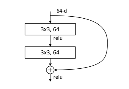
Residual learning, a building block. The first convolutional layer at the top takes a feature map with nxn pixels, each with 64 features. An identity shortcut copies the input data, which is summed with the output of the second convolutional layer.

If $x$ is the input image, we can think of the whole network function $G(x)$ as a composition of the functions of the $m$ building blocks,

$$G(x) = h_m (h_{m-1} (... h_1(x) ) ) $$

In classical networks, the identify shortcut does not exist, and block $i$ has to learn the function $h_i (x)$ directly. In ResNet, with the identity shortcut, we have

$$h_i(x) = f_i(x) + x$$

where f_i(x) is the residual function. In this way, the block only has to learn the residual function, which provides small deviations with respect to the input. The block does not have to reproduce its input anymore, in addition to modeling the small deviations.

Moreover, the addition of the identity shortcut does not increase the number of parameters of the block, because the identity shortcut has no parameter! It's just doing a copy.

As explained in the paper, it is this change that made it possible to create extremely deep networks. For example, the convolutional part of the ResNet50 network we're going to use has 50 layers, while VGG19 has 22. And there are also two even deeper versions of ResNet, ResNet101 and ResNet152.

At the same time, the number of parameters in ResNet50 is kept to a manageable 34 million, comparable to the 23 million parameters of VGG19! This is what makes it possible to learn a very deep representation rather easily from a "limited" dataset of about one million images.

So let's build a ResNet50 network with keras. First, we create our dataset iterators, with the right input shape and preprocessing functions

In [27]:
resnet50 = keras.applications.resnet50
train_dataset, val_dataset = generators((224,224), preprocessing=resnet50.preprocess_input)
Found 22481 images belonging to 2 classes.
Found 2496 images belonging to 2 classes.

Then, we create our full model, that is the convolutional part of ResNet50 followed by our simple classifier, the same as for VGG, and we train it.

In [28]:
conv_model = resnet50.ResNet50(weights='imagenet', include_top=False, input_shape=(224,224,3))
for layer in conv_model.layers:
    layer.trainable = False
x = keras.layers.Flatten()(conv_model.output)
x = keras.layers.Dense(100, activation='relu')(x)
predictions = keras.layers.Dense(2, activation='softmax')(x)
full_model = keras.models.Model(inputs=conv_model.input, outputs=predictions)
full_model.summary()
__________________________________________________________________________________________________
Layer (type)                    Output Shape         Param #     Connected to                     
==================================================================================================
input_7 (InputLayer)            (None, 224, 224, 3)  0                                            
__________________________________________________________________________________________________
conv1_pad (ZeroPadding2D)       (None, 230, 230, 3)  0           input_7[0][0]                    
__________________________________________________________________________________________________
conv1 (Conv2D)                  (None, 112, 112, 64) 9472        conv1_pad[0][0]                  
__________________________________________________________________________________________________
bn_conv1 (BatchNormalization)   (None, 112, 112, 64) 256         conv1[0][0]                      
__________________________________________________________________________________________________
activation_98 (Activation)      (None, 112, 112, 64) 0           bn_conv1[0][0]                   
__________________________________________________________________________________________________
pool1_pad (ZeroPadding2D)       (None, 114, 114, 64) 0           activation_98[0][0]              
__________________________________________________________________________________________________
max_pooling2d_2 (MaxPooling2D)  (None, 56, 56, 64)   0           pool1_pad[0][0]                  
__________________________________________________________________________________________________
res2a_branch2a (Conv2D)         (None, 56, 56, 64)   4160        max_pooling2d_2[0][0]            
__________________________________________________________________________________________________
bn2a_branch2a (BatchNormalizati (None, 56, 56, 64)   256         res2a_branch2a[0][0]             
__________________________________________________________________________________________________
activation_99 (Activation)      (None, 56, 56, 64)   0           bn2a_branch2a[0][0]              
__________________________________________________________________________________________________
res2a_branch2b (Conv2D)         (None, 56, 56, 64)   36928       activation_99[0][0]              
__________________________________________________________________________________________________
bn2a_branch2b (BatchNormalizati (None, 56, 56, 64)   256         res2a_branch2b[0][0]             
__________________________________________________________________________________________________
activation_100 (Activation)     (None, 56, 56, 64)   0           bn2a_branch2b[0][0]              
__________________________________________________________________________________________________
res2a_branch2c (Conv2D)         (None, 56, 56, 256)  16640       activation_100[0][0]             
__________________________________________________________________________________________________
res2a_branch1 (Conv2D)          (None, 56, 56, 256)  16640       max_pooling2d_2[0][0]            
__________________________________________________________________________________________________
bn2a_branch2c (BatchNormalizati (None, 56, 56, 256)  1024        res2a_branch2c[0][0]             
__________________________________________________________________________________________________
bn2a_branch1 (BatchNormalizatio (None, 56, 56, 256)  1024        res2a_branch1[0][0]              
__________________________________________________________________________________________________
add_32 (Add)                    (None, 56, 56, 256)  0           bn2a_branch2c[0][0]              
                                                                 bn2a_branch1[0][0]               
__________________________________________________________________________________________________
activation_101 (Activation)     (None, 56, 56, 256)  0           add_32[0][0]                     
__________________________________________________________________________________________________
res2b_branch2a (Conv2D)         (None, 56, 56, 64)   16448       activation_101[0][0]             
__________________________________________________________________________________________________
bn2b_branch2a (BatchNormalizati (None, 56, 56, 64)   256         res2b_branch2a[0][0]             
__________________________________________________________________________________________________
activation_102 (Activation)     (None, 56, 56, 64)   0           bn2b_branch2a[0][0]              
__________________________________________________________________________________________________
res2b_branch2b (Conv2D)         (None, 56, 56, 64)   36928       activation_102[0][0]             
__________________________________________________________________________________________________
bn2b_branch2b (BatchNormalizati (None, 56, 56, 64)   256         res2b_branch2b[0][0]             
__________________________________________________________________________________________________
activation_103 (Activation)     (None, 56, 56, 64)   0           bn2b_branch2b[0][0]              
__________________________________________________________________________________________________
res2b_branch2c (Conv2D)         (None, 56, 56, 256)  16640       activation_103[0][0]             
__________________________________________________________________________________________________
bn2b_branch2c (BatchNormalizati (None, 56, 56, 256)  1024        res2b_branch2c[0][0]             
__________________________________________________________________________________________________
add_33 (Add)                    (None, 56, 56, 256)  0           bn2b_branch2c[0][0]              
                                                                 activation_101[0][0]             
__________________________________________________________________________________________________
activation_104 (Activation)     (None, 56, 56, 256)  0           add_33[0][0]                     
__________________________________________________________________________________________________
res2c_branch2a (Conv2D)         (None, 56, 56, 64)   16448       activation_104[0][0]             
__________________________________________________________________________________________________
bn2c_branch2a (BatchNormalizati (None, 56, 56, 64)   256         res2c_branch2a[0][0]             
__________________________________________________________________________________________________
activation_105 (Activation)     (None, 56, 56, 64)   0           bn2c_branch2a[0][0]              
__________________________________________________________________________________________________
res2c_branch2b (Conv2D)         (None, 56, 56, 64)   36928       activation_105[0][0]             
__________________________________________________________________________________________________
bn2c_branch2b (BatchNormalizati (None, 56, 56, 64)   256         res2c_branch2b[0][0]             
__________________________________________________________________________________________________
activation_106 (Activation)     (None, 56, 56, 64)   0           bn2c_branch2b[0][0]              
__________________________________________________________________________________________________
res2c_branch2c (Conv2D)         (None, 56, 56, 256)  16640       activation_106[0][0]             
__________________________________________________________________________________________________
bn2c_branch2c (BatchNormalizati (None, 56, 56, 256)  1024        res2c_branch2c[0][0]             
__________________________________________________________________________________________________
add_34 (Add)                    (None, 56, 56, 256)  0           bn2c_branch2c[0][0]              
                                                                 activation_104[0][0]             
__________________________________________________________________________________________________
activation_107 (Activation)     (None, 56, 56, 256)  0           add_34[0][0]                     
__________________________________________________________________________________________________
res3a_branch2a (Conv2D)         (None, 28, 28, 128)  32896       activation_107[0][0]             
__________________________________________________________________________________________________
bn3a_branch2a (BatchNormalizati (None, 28, 28, 128)  512         res3a_branch2a[0][0]             
__________________________________________________________________________________________________
activation_108 (Activation)     (None, 28, 28, 128)  0           bn3a_branch2a[0][0]              
__________________________________________________________________________________________________
res3a_branch2b (Conv2D)         (None, 28, 28, 128)  147584      activation_108[0][0]             
__________________________________________________________________________________________________
bn3a_branch2b (BatchNormalizati (None, 28, 28, 128)  512         res3a_branch2b[0][0]             
__________________________________________________________________________________________________
activation_109 (Activation)     (None, 28, 28, 128)  0           bn3a_branch2b[0][0]              
__________________________________________________________________________________________________
res3a_branch2c (Conv2D)         (None, 28, 28, 512)  66048       activation_109[0][0]             
__________________________________________________________________________________________________
res3a_branch1 (Conv2D)          (None, 28, 28, 512)  131584      activation_107[0][0]             
__________________________________________________________________________________________________
bn3a_branch2c (BatchNormalizati (None, 28, 28, 512)  2048        res3a_branch2c[0][0]             
__________________________________________________________________________________________________
bn3a_branch1 (BatchNormalizatio (None, 28, 28, 512)  2048        res3a_branch1[0][0]              
__________________________________________________________________________________________________
add_35 (Add)                    (None, 28, 28, 512)  0           bn3a_branch2c[0][0]              
                                                                 bn3a_branch1[0][0]               
__________________________________________________________________________________________________
activation_110 (Activation)     (None, 28, 28, 512)  0           add_35[0][0]                     
__________________________________________________________________________________________________
res3b_branch2a (Conv2D)         (None, 28, 28, 128)  65664       activation_110[0][0]             
__________________________________________________________________________________________________
bn3b_branch2a (BatchNormalizati (None, 28, 28, 128)  512         res3b_branch2a[0][0]             
__________________________________________________________________________________________________
activation_111 (Activation)     (None, 28, 28, 128)  0           bn3b_branch2a[0][0]              
__________________________________________________________________________________________________
res3b_branch2b (Conv2D)         (None, 28, 28, 128)  147584      activation_111[0][0]             
__________________________________________________________________________________________________
bn3b_branch2b (BatchNormalizati (None, 28, 28, 128)  512         res3b_branch2b[0][0]             
__________________________________________________________________________________________________
activation_112 (Activation)     (None, 28, 28, 128)  0           bn3b_branch2b[0][0]              
__________________________________________________________________________________________________
res3b_branch2c (Conv2D)         (None, 28, 28, 512)  66048       activation_112[0][0]             
__________________________________________________________________________________________________
bn3b_branch2c (BatchNormalizati (None, 28, 28, 512)  2048        res3b_branch2c[0][0]             
__________________________________________________________________________________________________
add_36 (Add)                    (None, 28, 28, 512)  0           bn3b_branch2c[0][0]              
                                                                 activation_110[0][0]             
__________________________________________________________________________________________________
activation_113 (Activation)     (None, 28, 28, 512)  0           add_36[0][0]                     
__________________________________________________________________________________________________
res3c_branch2a (Conv2D)         (None, 28, 28, 128)  65664       activation_113[0][0]             
__________________________________________________________________________________________________
bn3c_branch2a (BatchNormalizati (None, 28, 28, 128)  512         res3c_branch2a[0][0]             
__________________________________________________________________________________________________
activation_114 (Activation)     (None, 28, 28, 128)  0           bn3c_branch2a[0][0]              
__________________________________________________________________________________________________
res3c_branch2b (Conv2D)         (None, 28, 28, 128)  147584      activation_114[0][0]             
__________________________________________________________________________________________________
bn3c_branch2b (BatchNormalizati (None, 28, 28, 128)  512         res3c_branch2b[0][0]             
__________________________________________________________________________________________________
activation_115 (Activation)     (None, 28, 28, 128)  0           bn3c_branch2b[0][0]              
__________________________________________________________________________________________________
res3c_branch2c (Conv2D)         (None, 28, 28, 512)  66048       activation_115[0][0]             
__________________________________________________________________________________________________
bn3c_branch2c (BatchNormalizati (None, 28, 28, 512)  2048        res3c_branch2c[0][0]             
__________________________________________________________________________________________________
add_37 (Add)                    (None, 28, 28, 512)  0           bn3c_branch2c[0][0]              
                                                                 activation_113[0][0]             
__________________________________________________________________________________________________
activation_116 (Activation)     (None, 28, 28, 512)  0           add_37[0][0]                     
__________________________________________________________________________________________________
res3d_branch2a (Conv2D)         (None, 28, 28, 128)  65664       activation_116[0][0]             
__________________________________________________________________________________________________
bn3d_branch2a (BatchNormalizati (None, 28, 28, 128)  512         res3d_branch2a[0][0]             
__________________________________________________________________________________________________
activation_117 (Activation)     (None, 28, 28, 128)  0           bn3d_branch2a[0][0]              
__________________________________________________________________________________________________
res3d_branch2b (Conv2D)         (None, 28, 28, 128)  147584      activation_117[0][0]             
__________________________________________________________________________________________________
bn3d_branch2b (BatchNormalizati (None, 28, 28, 128)  512         res3d_branch2b[0][0]             
__________________________________________________________________________________________________
activation_118 (Activation)     (None, 28, 28, 128)  0           bn3d_branch2b[0][0]              
__________________________________________________________________________________________________
res3d_branch2c (Conv2D)         (None, 28, 28, 512)  66048       activation_118[0][0]             
__________________________________________________________________________________________________
bn3d_branch2c (BatchNormalizati (None, 28, 28, 512)  2048        res3d_branch2c[0][0]             
__________________________________________________________________________________________________
add_38 (Add)                    (None, 28, 28, 512)  0           bn3d_branch2c[0][0]              
                                                                 activation_116[0][0]             
__________________________________________________________________________________________________
activation_119 (Activation)     (None, 28, 28, 512)  0           add_38[0][0]                     
__________________________________________________________________________________________________
res4a_branch2a (Conv2D)         (None, 14, 14, 256)  131328      activation_119[0][0]             
__________________________________________________________________________________________________
bn4a_branch2a (BatchNormalizati (None, 14, 14, 256)  1024        res4a_branch2a[0][0]             
__________________________________________________________________________________________________
activation_120 (Activation)     (None, 14, 14, 256)  0           bn4a_branch2a[0][0]              
__________________________________________________________________________________________________
res4a_branch2b (Conv2D)         (None, 14, 14, 256)  590080      activation_120[0][0]             
__________________________________________________________________________________________________
bn4a_branch2b (BatchNormalizati (None, 14, 14, 256)  1024        res4a_branch2b[0][0]             
__________________________________________________________________________________________________
activation_121 (Activation)     (None, 14, 14, 256)  0           bn4a_branch2b[0][0]              
__________________________________________________________________________________________________
res4a_branch2c (Conv2D)         (None, 14, 14, 1024) 263168      activation_121[0][0]             
__________________________________________________________________________________________________
res4a_branch1 (Conv2D)          (None, 14, 14, 1024) 525312      activation_119[0][0]             
__________________________________________________________________________________________________
bn4a_branch2c (BatchNormalizati (None, 14, 14, 1024) 4096        res4a_branch2c[0][0]             
__________________________________________________________________________________________________
bn4a_branch1 (BatchNormalizatio (None, 14, 14, 1024) 4096        res4a_branch1[0][0]              
__________________________________________________________________________________________________
add_39 (Add)                    (None, 14, 14, 1024) 0           bn4a_branch2c[0][0]              
                                                                 bn4a_branch1[0][0]               
__________________________________________________________________________________________________
activation_122 (Activation)     (None, 14, 14, 1024) 0           add_39[0][0]                     
__________________________________________________________________________________________________
res4b_branch2a (Conv2D)         (None, 14, 14, 256)  262400      activation_122[0][0]             
__________________________________________________________________________________________________
bn4b_branch2a (BatchNormalizati (None, 14, 14, 256)  1024        res4b_branch2a[0][0]             
__________________________________________________________________________________________________
activation_123 (Activation)     (None, 14, 14, 256)  0           bn4b_branch2a[0][0]              
__________________________________________________________________________________________________
res4b_branch2b (Conv2D)         (None, 14, 14, 256)  590080      activation_123[0][0]             
__________________________________________________________________________________________________
bn4b_branch2b (BatchNormalizati (None, 14, 14, 256)  1024        res4b_branch2b[0][0]             
__________________________________________________________________________________________________
activation_124 (Activation)     (None, 14, 14, 256)  0           bn4b_branch2b[0][0]              
__________________________________________________________________________________________________
res4b_branch2c (Conv2D)         (None, 14, 14, 1024) 263168      activation_124[0][0]             
__________________________________________________________________________________________________
bn4b_branch2c (BatchNormalizati (None, 14, 14, 1024) 4096        res4b_branch2c[0][0]             
__________________________________________________________________________________________________
add_40 (Add)                    (None, 14, 14, 1024) 0           bn4b_branch2c[0][0]              
                                                                 activation_122[0][0]             
__________________________________________________________________________________________________
activation_125 (Activation)     (None, 14, 14, 1024) 0           add_40[0][0]                     
__________________________________________________________________________________________________
res4c_branch2a (Conv2D)         (None, 14, 14, 256)  262400      activation_125[0][0]             
__________________________________________________________________________________________________
bn4c_branch2a (BatchNormalizati (None, 14, 14, 256)  1024        res4c_branch2a[0][0]             
__________________________________________________________________________________________________
activation_126 (Activation)     (None, 14, 14, 256)  0           bn4c_branch2a[0][0]              
__________________________________________________________________________________________________
res4c_branch2b (Conv2D)         (None, 14, 14, 256)  590080      activation_126[0][0]             
__________________________________________________________________________________________________
bn4c_branch2b (BatchNormalizati (None, 14, 14, 256)  1024        res4c_branch2b[0][0]             
__________________________________________________________________________________________________
activation_127 (Activation)     (None, 14, 14, 256)  0           bn4c_branch2b[0][0]              
__________________________________________________________________________________________________
res4c_branch2c (Conv2D)         (None, 14, 14, 1024) 263168      activation_127[0][0]             
__________________________________________________________________________________________________
bn4c_branch2c (BatchNormalizati (None, 14, 14, 1024) 4096        res4c_branch2c[0][0]             
__________________________________________________________________________________________________
add_41 (Add)                    (None, 14, 14, 1024) 0           bn4c_branch2c[0][0]              
                                                                 activation_125[0][0]             
__________________________________________________________________________________________________
activation_128 (Activation)     (None, 14, 14, 1024) 0           add_41[0][0]                     
__________________________________________________________________________________________________
res4d_branch2a (Conv2D)         (None, 14, 14, 256)  262400      activation_128[0][0]             
__________________________________________________________________________________________________
bn4d_branch2a (BatchNormalizati (None, 14, 14, 256)  1024        res4d_branch2a[0][0]             
__________________________________________________________________________________________________
activation_129 (Activation)     (None, 14, 14, 256)  0           bn4d_branch2a[0][0]              
__________________________________________________________________________________________________
res4d_branch2b (Conv2D)         (None, 14, 14, 256)  590080      activation_129[0][0]             
__________________________________________________________________________________________________
bn4d_branch2b (BatchNormalizati (None, 14, 14, 256)  1024        res4d_branch2b[0][0]             
__________________________________________________________________________________________________
activation_130 (Activation)     (None, 14, 14, 256)  0           bn4d_branch2b[0][0]              
__________________________________________________________________________________________________
res4d_branch2c (Conv2D)         (None, 14, 14, 1024) 263168      activation_130[0][0]             
__________________________________________________________________________________________________
bn4d_branch2c (BatchNormalizati (None, 14, 14, 1024) 4096        res4d_branch2c[0][0]             
__________________________________________________________________________________________________
add_42 (Add)                    (None, 14, 14, 1024) 0           bn4d_branch2c[0][0]              
                                                                 activation_128[0][0]             
__________________________________________________________________________________________________
activation_131 (Activation)     (None, 14, 14, 1024) 0           add_42[0][0]                     
__________________________________________________________________________________________________
res4e_branch2a (Conv2D)         (None, 14, 14, 256)  262400      activation_131[0][0]             
__________________________________________________________________________________________________
bn4e_branch2a (BatchNormalizati (None, 14, 14, 256)  1024        res4e_branch2a[0][0]             
__________________________________________________________________________________________________
activation_132 (Activation)     (None, 14, 14, 256)  0           bn4e_branch2a[0][0]              
__________________________________________________________________________________________________
res4e_branch2b (Conv2D)         (None, 14, 14, 256)  590080      activation_132[0][0]             
__________________________________________________________________________________________________
bn4e_branch2b (BatchNormalizati (None, 14, 14, 256)  1024        res4e_branch2b[0][0]             
__________________________________________________________________________________________________
activation_133 (Activation)     (None, 14, 14, 256)  0           bn4e_branch2b[0][0]              
__________________________________________________________________________________________________
res4e_branch2c (Conv2D)         (None, 14, 14, 1024) 263168      activation_133[0][0]             
__________________________________________________________________________________________________
bn4e_branch2c (BatchNormalizati (None, 14, 14, 1024) 4096        res4e_branch2c[0][0]             
__________________________________________________________________________________________________
add_43 (Add)                    (None, 14, 14, 1024) 0           bn4e_branch2c[0][0]              
                                                                 activation_131[0][0]             
__________________________________________________________________________________________________
activation_134 (Activation)     (None, 14, 14, 1024) 0           add_43[0][0]                     
__________________________________________________________________________________________________
res4f_branch2a (Conv2D)         (None, 14, 14, 256)  262400      activation_134[0][0]             
__________________________________________________________________________________________________
bn4f_branch2a (BatchNormalizati (None, 14, 14, 256)  1024        res4f_branch2a[0][0]             
__________________________________________________________________________________________________
activation_135 (Activation)     (None, 14, 14, 256)  0           bn4f_branch2a[0][0]              
__________________________________________________________________________________________________
res4f_branch2b (Conv2D)         (None, 14, 14, 256)  590080      activation_135[0][0]             
__________________________________________________________________________________________________
bn4f_branch2b (BatchNormalizati (None, 14, 14, 256)  1024        res4f_branch2b[0][0]             
__________________________________________________________________________________________________
activation_136 (Activation)     (None, 14, 14, 256)  0           bn4f_branch2b[0][0]              
__________________________________________________________________________________________________
res4f_branch2c (Conv2D)         (None, 14, 14, 1024) 263168      activation_136[0][0]             
__________________________________________________________________________________________________
bn4f_branch2c (BatchNormalizati (None, 14, 14, 1024) 4096        res4f_branch2c[0][0]             
__________________________________________________________________________________________________
add_44 (Add)                    (None, 14, 14, 1024) 0           bn4f_branch2c[0][0]              
                                                                 activation_134[0][0]             
__________________________________________________________________________________________________
activation_137 (Activation)     (None, 14, 14, 1024) 0           add_44[0][0]                     
__________________________________________________________________________________________________
res5a_branch2a (Conv2D)         (None, 7, 7, 512)    524800      activation_137[0][0]             
__________________________________________________________________________________________________
bn5a_branch2a (BatchNormalizati (None, 7, 7, 512)    2048        res5a_branch2a[0][0]             
__________________________________________________________________________________________________
activation_138 (Activation)     (None, 7, 7, 512)    0           bn5a_branch2a[0][0]              
__________________________________________________________________________________________________
res5a_branch2b (Conv2D)         (None, 7, 7, 512)    2359808     activation_138[0][0]             
__________________________________________________________________________________________________
bn5a_branch2b (BatchNormalizati (None, 7, 7, 512)    2048        res5a_branch2b[0][0]             
__________________________________________________________________________________________________
activation_139 (Activation)     (None, 7, 7, 512)    0           bn5a_branch2b[0][0]              
__________________________________________________________________________________________________
res5a_branch2c (Conv2D)         (None, 7, 7, 2048)   1050624     activation_139[0][0]             
__________________________________________________________________________________________________
res5a_branch1 (Conv2D)          (None, 7, 7, 2048)   2099200     activation_137[0][0]             
__________________________________________________________________________________________________
bn5a_branch2c (BatchNormalizati (None, 7, 7, 2048)   8192        res5a_branch2c[0][0]             
__________________________________________________________________________________________________
bn5a_branch1 (BatchNormalizatio (None, 7, 7, 2048)   8192        res5a_branch1[0][0]              
__________________________________________________________________________________________________
add_45 (Add)                    (None, 7, 7, 2048)   0           bn5a_branch2c[0][0]              
                                                                 bn5a_branch1[0][0]               
__________________________________________________________________________________________________
activation_140 (Activation)     (None, 7, 7, 2048)   0           add_45[0][0]                     
__________________________________________________________________________________________________
res5b_branch2a (Conv2D)         (None, 7, 7, 512)    1049088     activation_140[0][0]             
__________________________________________________________________________________________________
bn5b_branch2a (BatchNormalizati (None, 7, 7, 512)    2048        res5b_branch2a[0][0]             
__________________________________________________________________________________________________
activation_141 (Activation)     (None, 7, 7, 512)    0           bn5b_branch2a[0][0]              
__________________________________________________________________________________________________
res5b_branch2b (Conv2D)         (None, 7, 7, 512)    2359808     activation_141[0][0]             
__________________________________________________________________________________________________
bn5b_branch2b (BatchNormalizati (None, 7, 7, 512)    2048        res5b_branch2b[0][0]             
__________________________________________________________________________________________________
activation_142 (Activation)     (None, 7, 7, 512)    0           bn5b_branch2b[0][0]              
__________________________________________________________________________________________________
res5b_branch2c (Conv2D)         (None, 7, 7, 2048)   1050624     activation_142[0][0]             
__________________________________________________________________________________________________
bn5b_branch2c (BatchNormalizati (None, 7, 7, 2048)   8192        res5b_branch2c[0][0]             
__________________________________________________________________________________________________
add_46 (Add)                    (None, 7, 7, 2048)   0           bn5b_branch2c[0][0]              
                                                                 activation_140[0][0]             
__________________________________________________________________________________________________
activation_143 (Activation)     (None, 7, 7, 2048)   0           add_46[0][0]                     
__________________________________________________________________________________________________
res5c_branch2a (Conv2D)         (None, 7, 7, 512)    1049088     activation_143[0][0]             
__________________________________________________________________________________________________
bn5c_branch2a (BatchNormalizati (None, 7, 7, 512)    2048        res5c_branch2a[0][0]             
__________________________________________________________________________________________________
activation_144 (Activation)     (None, 7, 7, 512)    0           bn5c_branch2a[0][0]              
__________________________________________________________________________________________________
res5c_branch2b (Conv2D)         (None, 7, 7, 512)    2359808     activation_144[0][0]             
__________________________________________________________________________________________________
bn5c_branch2b (BatchNormalizati (None, 7, 7, 512)    2048        res5c_branch2b[0][0]             
__________________________________________________________________________________________________
activation_145 (Activation)     (None, 7, 7, 512)    0           bn5c_branch2b[0][0]              
__________________________________________________________________________________________________
res5c_branch2c (Conv2D)         (None, 7, 7, 2048)   1050624     activation_145[0][0]             
__________________________________________________________________________________________________
bn5c_branch2c (BatchNormalizati (None, 7, 7, 2048)   8192        res5c_branch2c[0][0]             
__________________________________________________________________________________________________
add_47 (Add)                    (None, 7, 7, 2048)   0           bn5c_branch2c[0][0]              
                                                                 activation_143[0][0]             
__________________________________________________________________________________________________
activation_146 (Activation)     (None, 7, 7, 2048)   0           add_47[0][0]                     
__________________________________________________________________________________________________
flatten_4 (Flatten)             (None, 100352)       0           activation_146[0][0]             
__________________________________________________________________________________________________
dense_16 (Dense)                (None, 100)          10035300    flatten_4[0][0]                  
__________________________________________________________________________________________________
dense_17 (Dense)                (None, 100)          10100       dense_16[0][0]                   
__________________________________________________________________________________________________
dense_18 (Dense)                (None, 100)          10100       dense_17[0][0]                   
__________________________________________________________________________________________________
dense_19 (Dense)                (None, 2)            202         dense_18[0][0]                   
==================================================================================================
Total params: 33,643,414
Trainable params: 10,055,702
Non-trainable params: 23,587,712
__________________________________________________________________________________________________
In [29]:
full_model.compile(loss='binary_crossentropy',
                  optimizer=keras.optimizers.Adamax(lr=0.001),
                  metrics=['acc'])
history = full_model.fit_generator(
    train_dataset, 
    validation_data = val_dataset,
    workers=10,
    epochs=5,
)
Epoch 1/5
750/750 [==============================] - 64s 85ms/step - loss: 0.1398 - acc: 0.9616 - val_loss: 0.0328 - val_acc: 0.9872
Epoch 2/5
750/750 [==============================] - 60s 80ms/step - loss: 0.0509 - acc: 0.9821 - val_loss: 0.0354 - val_acc: 0.9892
Epoch 3/5
750/750 [==============================] - 60s 80ms/step - loss: 0.0431 - acc: 0.9851 - val_loss: 0.0908 - val_acc: 0.9780
Epoch 4/5
750/750 [==============================] - 61s 82ms/step - loss: 0.0326 - acc: 0.9893 - val_loss: 0.0443 - val_acc: 0.9868
Epoch 5/5
750/750 [==============================] - 61s 81ms/step - loss: 0.0212 - acc: 0.9918 - val_loss: 0.0597 - val_acc: 0.9860
In [30]:
plot_history(history, yrange=(0.9,1))

Saving and loading a Keras model

Let's say you obtained excellent performance with a given model. You certainly want to save this model for future use. Let's do this now with our model based on ResNet50, which is the last one we have trained.

With Keras, it's possible to make the full model persistent on disk, but the models might become unreadable when non-standard layers are used.

I find saving only the model weights (parameters) easier:

In [33]:
full_model.save_weights('resnet50.h5')

To read them again, we create a new model, identical to the one we have trained:

In [24]:
conv_model = resnet50.ResNet50(weights='imagenet', include_top=False, input_shape=(224,224,3))
for layer in conv_model.layers:
    layer.trainable = False
x = keras.layers.Flatten()(conv_model.output)
x = keras.layers.Dense(100, activation='relu')(x)
predictions = keras.layers.Dense(2, activation='softmax')(x)
full_model = keras.models.Model(inputs=conv_model.input, outputs=predictions)

And we load the weights:

In [25]:
full_model.load_weights('resnet50.h5')

Model evaluation

We can start by evaluating a single image (note that we are now using the model that has been saved and reloaded):

In [31]:
from keras.preprocessing import image
from keras.applications.resnet50 import preprocess_input

img_path = 'dogs/dog.1.jpg'
img = image.load_img(img_path, target_size=(224,224))
x = image.img_to_array(img)
x = np.expand_dims(x, axis=0)
x = preprocess_input(x)
print(full_model.predict(x))
plt.imshow(img)
[[9.9993050e-01 6.9532914e-05]]
Out[31]:
<matplotlib.image.AxesImage at 0x7f1ebf61e400>

Our neural network gives this image a whopping 99.993% probability. That's actually not too surprising: this is an archetypal dog, so no difficulty here.

But what about other images in the dataset? It would be very interesting to look at misidentified images, to see what's going on with them. Let's start by evaluating the model for all images in the training dataset:

In [49]:
import sys

def true_and_predicted_labels(dataset):
    labels = np.zeros((dataset.n,2))
    preds = np.zeros_like(labels)
    for i in range(len(dataset)):
        sys.stdout.write('evaluating batch {}\r'.format(i))
        sys.stdout.flush()
        batch = dataset[i]
        batch_images = batch[0]
        batch_labels = batch[1]
        batch_preds = full_model.predict(batch_images)
        start = i*batch_size
        labels[start:start+batch_size] = batch_labels
        preds[start:start+batch_size] = batch_preds
    return labels, preds

train_labels, train_preds = true_and_predicted_labels(train_dataset)
evaluating batch 749

Now that we have the model predictions, we can illustrate how the model is able to separate the two categories. For this, we will consider only the cat score, remembering that the dog score is equal to one minus the cat score. And we will plot the cat score for the two categories. For cats, we expect the cat score to be close to one. For dogs, it will be close to zero.

In [50]:
def plot_cat_score(preds, labels, range=(0,1)):
    # get the cat score for all images
    cat_score = preds[:,1]
    # get the cat score for dogs
    # we use the true labels to select dog images
    dog_cat_score = cat_score[labels[:,0]>0.5]
    # and for cats
    cat_cat_score = cat_score[labels[:,0]<0.5]
    # just some plotting parameters
    params = {'bins':100, 'range':range, 'alpha':0.6}
    plt.hist(dog_cat_score, **params)
    plt.hist(cat_cat_score, **params)
    plt.yscale('log')
In [51]:
plot_cat_score(train_preds, train_labels)

Please note that I have used a log scale on the y axis. I did this because, with this excellent classification accuracy, we end up with most pictures having either a cat score very close to 1 (clear cats), or very close to 0 (clear dogs), such as the example we plotted above. We would only see these in linear scale. In the middle, we see the more difficult and interesting cases.

We can now compute the accuracy.

For this we need to compute the predicted labels and compare them with the true labels. To compute the predicted labels, we take the cat score, and we decide that the network predicts a cat if this score is larger than a given threshold.

Keras provides an estimation of the accuracy during the training. For this estimation, keras uses a threshold of 0.5, so let's do that as well:

In [52]:
threshold = 0.5

def predicted_labels(preds, threshold):
    '''Turn predictions (floats in the last two dimensions) 
    into labels (0 or 1).'''
    pred_labels = np.zeros_like(preds)
    # cat score lower than threshold: set dog label to 1
    # cat score higher than threshold: set dog label to 0
    pred_labels[:,0] = preds[:,1]<threshold
    # cat score higher than threshold: set cat label to 1
    # cat score lower than threshold: set cat label to 0
    pred_labels[:,1] = preds[:,1]>=threshold
    return pred_labels

train_pred_labels = predicted_labels(train_preds, threshold)
print('predicted labels:')
print(train_pred_labels)
print('true labels:')
print(train_labels)
predicted labels:
[[1. 0.]
 [1. 0.]
 [0. 1.]
 ...
 [1. 0.]
 [0. 1.]
 [1. 0.]]
true labels:
[[1. 0.]
 [1. 0.]
 [0. 1.]
 ...
 [1. 0.]
 [0. 1.]
 [1. 0.]]

We see that the predicted labels seem to be very similar to the true labels. This is because the accuracy is close to 100%, and only a few examples are shown in the printout above. Let's quantify the fraction of misclassified examples:

In [61]:
def misclassified(labels, pred_labels, print_report=True):
    def report(categ, n_misclassified, n_examples): 
        print('{:<4} {:>3} misclassified samples ({:4.2f}%)'.format(
            categ,
            n_misclassified, 
            100*(1-float(n_misclassified)/n_examples))
        )
    # total number of examples
    n_examples = len(labels)
    # total number of cats
    n_cats = sum(labels[:,0])
    # total number of dogs
    n_dogs = sum(labels[:,1])
    # boolean mask for misidentified examples
    mask_all = pred_labels[:,0] != labels[:,0]
    # boolean mask for misidentified cats    
    mask_cats = np.logical_and(mask_all,labels[:,1]>0.5)
    # boolean mask for misidentified dogs    
    mask_dogs = np.logical_and(mask_all,labels[:,1]<0.5)
    if print_report:
        report('all', sum(mask_all), n_examples)
        report('cats', sum(mask_cats), n_cats)
        report('dogs', sum(mask_dogs), n_dogs)
    return mask_all, mask_cats, mask_dogs

_ = misclassified(train_labels, train_pred_labels)
all  104 misclassified samples (99.54%)
cats  23 misclassified samples (99.80%)
dogs  81 misclassified samples (99.28%)

With my training, we see that the dogs are more difficult to classify. However, each training could lead to different results. I did a few, and I got symmetric classification performance only once.

Now, is there a reason to pick a threshold at 0.5 for classification? Let's plot the cat score again:

In [64]:
plot_cat_score(train_preds, train_labels)

Clearly, with a threshold of 0.9 or so, we are only going to misclassify a few more cats, but we will gain a lot of dogs. After a bit of optimization, we reach symmetric classification with a threshold of 0.85:

In [69]:
threshold = 0.85
train_pred_labels = predicted_labels(train_preds, threshold)
_ = misclassified(train_labels, train_pred_labels)
all  100 misclassified samples (99.56%)
cats  50 misclassified samples (99.56%)
dogs  50 misclassified samples (99.56%)

With this choice of threshold, we improve the global classification accuracy by 0.02%. That's not a big gain in this case, but remember that depending on the training, you might get much more asymmetrical distributions. You can try retraining ResNet50 again to check this.

So remember:


Check the classification score and tune your threshold properly.


Now, we optimized the threshold on the training dataset. What do we get with the validation dataset?

In [70]:
val_labels, val_preds = true_and_predicted_labels(val_dataset)
val_pred_labels = predicted_labels(val_preds, threshold)
_ = misclassified(val_labels, val_pred_labels)
all   35 misclassified samples (98.60%)
cats  17 misclassified samples (98.64%)
dogs  18 misclassified samples (98.56%)

Here also, the classification is rather symmetric, and the validation accuracy is 98.6%. With a classification threshold at 0.5, we would get:

In [71]:
val_pred_labels = predicted_labels(val_preds, 0.5)
_ = misclassified(val_labels, val_pred_labels)
all   38 misclassified samples (98.48%)
cats  12 misclassified samples (99.04%)
dogs  26 misclassified samples (97.92%)

Looking at misclassified pictures

There is a slight issue in the interface of the ImageDataGenerator : it does not allow us to find back the images that are misclassified, so that we could load them from disk and look at them. So we need to evaluate again the network again, storing the misidentified images for later display.

In [74]:
import sys

dataset = val_dataset
misclassified_imgs = dict(dogs=[], cats=[])
for i in range(len(dataset)):
    if i%100: 
        sys.stdout.write('evaluating batch {}\r'.format(i))
        sys.stdout.flush()
    batch = dataset[i]
    batch_images = batch[0]
    batch_labels = batch[1]
    batch_preds = full_model.predict(batch_images)
    batch_pred_labels = predicted_labels(batch_preds, threshold=0.85)
    mask_all, mask_cats, mask_dogs = misclassified(
        batch_labels, 
        batch_pred_labels,
        print_report=False                                  
    )
    misclassified_imgs['dogs'].extend(batch_images[mask_dogs])
    misclassified_imgs['cats'].extend(batch_images[mask_cats])
evaluating batch 83

Here is the number of misclassified images in each category:

In [75]:
print([(label, len(imgs)) for label,imgs in misclassified_imgs.items()])
[('dogs', 14), ('cats', 18)]

You have certainly noticed that these numbers do not correspond exactly to the ones we have seen above (17 misclassified cats and 18 misclassified dogs). I think this might be due to some amount of randomness in the evaluation of the network, or to numerical precision, and I have no idea where this is coming from.

Now let's write a small function to plot a bunch of images, so that we can have a look at the misclassified images:

In [76]:
def plot_images(imgs, i):
    ncols, nrows = (5, 2) 
    start = i*ncols*nrows
    fig = plt.figure( figsize=(ncols*5, nrows*5), dpi=50)
    for i, img in enumerate(imgs[start:start+ncols*nrows]):
        plt.subplot(nrows, ncols, i+1)
        plt.imshow(img)
        plt.axis('off')
In [77]:
plot_images(misclassified_imgs['cats'],0)
Clipping input data to the valid range for imshow with RGB data ([0..1] for floats or [0..255] for integers).

Wow what's this?? the colors are completely messed up...

This is due to the image preprocessing performed by the dataset iterator. Remember that we're using ResNet50 and that have requested our images to be preprocessed with keras.applications.resnet50.preprocess_input . Do we have a way to undo this operation? For that we first need to find this function to understand what it is doing.

We start by checking our version of keras_applications :

In [78]:
import keras_applications
keras_applications.__version__
Out[78]:
'1.0.8'

Then we look at the source code of resnet50 and we see that this function is taken from imagenet_utils , where it is defined here .

We're calling the function without any argument apart from the image to be preprocessed. So we're in "caffe" mode. Also, we are providing a numpy array to the function, so we are actually calling _preprocess_numpy_input , here .

In the caffe mode, the function is doing the following:

  • switch from the RGB color representation to BGR
  • subtract the mean BGR values calculated for the whole ImageNet dataset to center the BGR values on 0

We can easily write a function to undo this operation:

In [79]:
def undo_preprocessing(x):
    mean = [103.939, 116.779, 123.68]
    x[..., 0] += mean[0]
    x[..., 1] += mean[1]
    x[..., 2] += mean[2]
    x = x[..., ::-1]

Our function first adds back the mean of the BGR values, since this was the last operation of the preprocessing. And then we revert again the order of the color levels. What might not be obvious to you is the last line, which reverts the order of the color levels. So let's have a look in details.

  • the notation ... means: add as many dimensions as necessary. So we're going to leave the first dimensions of the images untouched, to act only on the last dimension, the one of the color levels (please note that I'm using keras in channels last mode).
  • the notation ::-1 acts on the last dimension, and revert the order of the numbers there.

Let's take a simple example. We build an array with shape (2,2,3). You can think of it as an image with 2x2 pixels and 3 color levels:

In [80]:
a = np.arange(12).reshape(2,2,3)
print(a)
[[[ 0  1  2]
  [ 3  4  5]]

 [[ 6  7  8]
  [ 9 10 11]]]

In the top left pixel, the three color levels are set to [0 1 2] respectively, and in the bottom right pixel to [9 10 11] . We can see that the reverting operation has the expected effect:

In [81]:
a[...,::-1]
Out[81]:
array([[[ 2,  1,  0],
        [ 5,  4,  3]],

       [[ 8,  7,  6],
        [11, 10,  9]]])

Now let's try our unprocessing function on one image:

In [83]:
img = misclassified_imgs['cats'][5]
plt.imshow(img)
Clipping input data to the valid range for imshow with RGB data ([0..1] for floats or [0..255] for integers).
Out[83]:
<matplotlib.image.AxesImage at 0x7f1e9c3e04e0>
In [84]:
import copy
new_img = copy.copy(img)
undo_preprocessing(new_img)
plt.imshow(new_img.astype('int'))
Out[84]:
<matplotlib.image.AxesImage at 0x7f1e9c3406d8>

Much better! The function seems to work as expected. So we modify our plotting function to plot unprocessed images:

In [85]:
def plot_images(imgs, i):
    ncols, nrows = (5, 2) 
    start = i*ncols*nrows
    fig = plt.figure( figsize=(ncols*5, nrows*5), dpi=50)
    for i, img in enumerate(imgs[start:start+ncols*nrows]):
        img_unproc = copy.copy(img)
        undo_preprocessing(img_unproc)
        plt.subplot(nrows, ncols, i+1)
        plt.imshow(img_unproc.astype('int'))
        plt.axis('off')
In [86]:
plot_images(misclassified_imgs['dogs'],0)

Actually the colors still look a bit funny... I don't really know why and being colorblind, I'm not completely sure! Anyway, we can at least understand the images now.

We can try to guess why these images were misclassified. It could be that cats are more often carried by people, which would bias the network towards misclassifying dogs when people are in the image. Also, the wrong orientation of one image probably does not help. Then, cats often sleep on their back, while this position is not that common for dogs. Finally, puppies are certainly more challenging.

Conclusion and outlook

In this post, you learnt what is transfer learning and how to:

  • use the VGG16, VGG19, and ResNet50 pre-trained models in keras, to reach a 98.5% accuracy on dog vs cat classification.
  • add layers to an existing model to adapt it to your needs
  • save a keras model so that you can re-use it later on, without having to retrain.
  • create your own tools to evaluate the model performance and have a look at misidentified pictures, with python and numpy.

What now?

Deep neural networks trained on the large ImageNet dataset can see! And we can use them to classify images in different categories, and with smaller dataset.

So let's say you have your own set of images that you'd like to classify. Maybe you want to identify mushrooms? or insects? or find out whether a medical image is suspicious? Transfer learning is probably the way to go.

Next, we'll build a dataset from scratch by collecting images on the internet. With this dataset, we will be able to test our transfer learning skills on different, yet unknown categories. After all, ImageNet features dogs and cats).

And we will also study transfer learning in the context of natural language processing.


Please let me know what you think in the comments! I’ll try and answer all questions.

And if you liked this article, you can subscribe to my mailing list to be notified of new posts (no more than one mail per week I promise.)

Back Home