CUDA kernels in python
Write your own CUDA kernels in python to accelerate your computing on the GPU. Notebook ready to run on the Google Colab platform
Introduction
In this post, you will learn how to write your own custom CUDA kernels to do accelerated, parallel computing on a GPU, in python with the help of numba and CUDA.
We will use the Google Colab platform, so you don't even need to own a GPU to run this tutorial.
This is the third part of my series on accelerated computing with python:
- Part I : Make python fast with numba : accelerated python on the CPU
- Part II : Boost python with your GPU (numba+CUDA)
- Part III : Custom CUDA kernels with numba+CUDA
- Part IV : Parallel processing with dask (to be written)
In part II , we have seen how to vectorize a calculation on the GPU. But what does this mean?
Let's consider an array of values, and assume that we need to perform a given operation on each element of the array. For example, we might want to compute the square root of each element in the array.
In classical, sequential programming, we would write a loop to do that. Vectorization consists in rewriting the loop in such a way as to process the elements of the array in parallel. For example, if the array is of size 100, we could use 5 threads working at the same time, each processing 20 elements.
In other words, we take a scalar operation (e.g. computing the square root of a single value), and turn it into a vector operation (e.g. computing the square root of all elements in the array).
A wide variety of problems can be vectorized, and we have seen how to do that easily in python with the vectorize decorator provided by numba.
But in some cases, simple vectorization is not possible. For example, let's consider the Gaussian blur algorithm, which can be used to smooth an image and is often used to remove noise in photos. Each pixel in the output image is computed by averaging neighbouring pixels in the input image.

It's not possible to vectorize the Gaussian blur algorithm, as we need to consider more than one input values to compute the output value. However, we can still run such an algorithm in parallel on a GPU by writing a custom CUDA kernel.
In this article, you will:
- understand the differences between the GPU and CPU architecture;
- implement a very simple CUDA kernel, just to get started;
- learn how to write more efficient code with striding;
- deal with two-dimensional datasets, performing matrix multiplication on the GPU.
A few parts of this article have been taken from the very nice (but private) DLI tutorial from nvidia.
GPU and CPU architectures
GPU development has been driven by the demand for high-definition 3D graphics for almost two decades. To process a very large number of pixels at high speed, GPUs evolved into massively parallel processors with huge computing power and memory bandwidth.
The main differences between the GPU and CPU architectures are outlined in the introduction of the CUDA C programming guide . In a schematic way:

GPU clock speeds are typically three times lower than CPU clock speeds. But this is vastly compensated by the much larger number of computing cores:
| Base Clock speed | Number of cores | |
| Tesla V100 GPU | 1.45 GHz | 5120 |
| Intel Core i9-9900K | 3.6 GHz | 8 |
To leverage the tremendous power of the GPU, it is however necessary to adopt a new programming paradigm.
Indeed, on the CPU, we process a large amount of data sequentially, basically looping over the data. On the GPU, we need to split the processing into elementary tasks that only deal with a small fraction of the data. These tasks (or threads) can then be handled in parallel by the many cores of the GPU.
As you will see, writing an algorithm for the GPU is not that difficult thanks to the CUDA parallel programming model.
You can execute the code below in a jupyter notebook on the Google Colab platform by simply following this link . Open it in Chrome rather than Firefox, and make sure to select GPU as execution environment.
But you can also just keep reading through here if you prefer!
Numba + CUDA on Google Colab 
By default, Google Colab is not able to run numba + CUDA, because two libraries are not found,
libdevice
and
libnvvm.so
. So we need to make sure that these libraries are found in the notebook.
First, we look for these libraries on the system. To do that, we simply run the
find
command, to recursively look for these libraries starting at the root of the filesystem. The exclamation mark escapes the line so that it's executed by the Linux shell, and not by the jupyter notebook.
!find / -iname 'libdevice'
!find / -iname 'libnvvm.so'
Then, we add the two libraries to numba environment variables:
import os
os.environ['NUMBAPRO_LIBDEVICE'] = "/usr/local/cuda-10.0/nvvm/libdevice"
os.environ['NUMBAPRO_NVVM'] = "/usr/local/cuda-10.0/nvvm/lib64/libnvvm.so"
And we're done!
A very simple CUDA kernel 
Let's get started by implementing a first CUDA kernel to compute the square root of each value in an array. First, here is our array:
import numpy as np
a = np.arange(4096,dtype=np.float32)
a
As we have seen in part II , and as discussed in the introduction, we can simply use numba's vectorize decorator to compute the square root of all elements in parallel on the GPU:
import math
from numba import vectorize

@vectorize(['float32(float32)'], target='cuda')
def gpu_sqrt(x):
    return math.sqrt(x)

gpu_sqrt(a)
This time, as an exercise, we'll do the same with a custom CUDA kernel.
We first define our kernel:
from numba import cuda

@cuda.jit
def gpu_sqrt_kernel(x, out):
  idx = cuda.grid(1)
  out[idx] = math.sqrt(x[idx])
Let's discuss this code in some details.
We have an input array of 4096 values, so we will use 4096 threads on the GPU.
Our input and output arrays are one dimensional, so we will use a one-dimensional
grid
of threads (we will discuss grids in details in the next section). The call
cuda.grid(1)
returns the unique index for the current thread in the whole grid. With 4096 threads,
idx
will range from 0 to 4095.
Then, we see in the code that each thread is going to deal with a single element of the input array to produce a single element in the output array. This element is determined for each thread by the thread index.
Now that we have our kernel, we copy our input array to the GPU device, create an output array on the device with the same shape, and finally launch the kernel:
# move input data to the device
d_a = cuda.to_device(a)
# create output data on the device
d_out = cuda.device_array_like(d_a)

# we decide to use 32 blocks, each containing 128 threads
blocks_per_grid = 32
threads_per_block = 128
gpu_sqrt_kernel[blocks_per_grid, threads_per_block](d_a, d_out)
# wait for all threads to complete
cuda.synchronize()
# copy the output array back to the host system
# and print it
print(d_out.copy_to_host())
In the code above, the 4096 threads are arranged into a grid of 32 blocks , each block having 128 threads. This execution configuration will be discussed in the next section.
Exercises:
- Go back to the previous cell, and try to decrease the number of blocks per grid, or the number of threads per block.
- Then try to increase the number of blocks per grid, or the number of threads per blocks
-
Try to remove the
cuda.synchronize()call
Results :
- When you reduce the number of threads, either by decreasing the number of blocks per grid or the number of threads per block, some elements are not processed, and the corresponding slots at the end of the output array remain set to their default value, which is 0.
- If, on the other hand, you increase the number of threads, it seems that everything is working fine. However, this actually creates an error even though we cannot see it. We will see later how to expose this error. Debugging code is one of the difficulties of CUDA, as the error messages are not always visible.
-
Finally, you might have expected that commenting out the call to
cuda.synchronizewould have resulted in output array only partially filled, or not filled at all. That would be a good guess since the CPU keeps running the main program (the one of the cell) while the GPU processes the data asynchronously. However, the copy to the host performs an implicit synchronization, so the call to cuda.syncronize is not necessary.
Execution configuration : number of blocks and number of threads 
In our first example above, we decided to use 4096 threads. These threads were arranged as a grid containing 32 blocks of 128 threads each.
You probably wondered why we decided to do that. So in this section, I will try and answer some of the questions you may have:
- Why do we need to arrange threads into blocks within the grid?
- How did we come up with the magical numbers 32 and 128? Could we use other values like 16 and 256 (which still total 4096), or 64 and 64?
These questions are important if you care about performance -- and you probably do if you're here to learn how to speed up your calculations on a GPU! To answer these questions, we first need to learn about our GPU hardware.
CUDA: Learn about your GPU hardware 
Let's find out about the GPU we are using. Please note that your GPU (or the GPU attributed to you on Google Colab) could be different from mine. Of course, the numbers I'm giving below and the picture are only valid for the GPU attributed to me during my session on Google Colab.
cuda.detect()
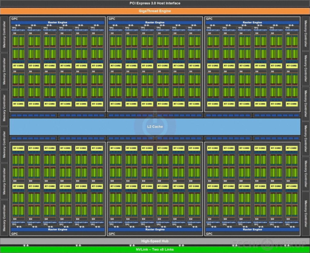
We see that's an nvidia T4 , and here is the white paper with the specs for the Turing architecture. In this paper, we see that the T4 is based on the Turing TU102 GPU which has:
- 72 streaming multiprocessors
- 64 cuda cores per streaming multiprocessor
Here is a block diagram of the TU102 GPU. The streaming multiprocessors are the 72 inner blocks labelled SM.
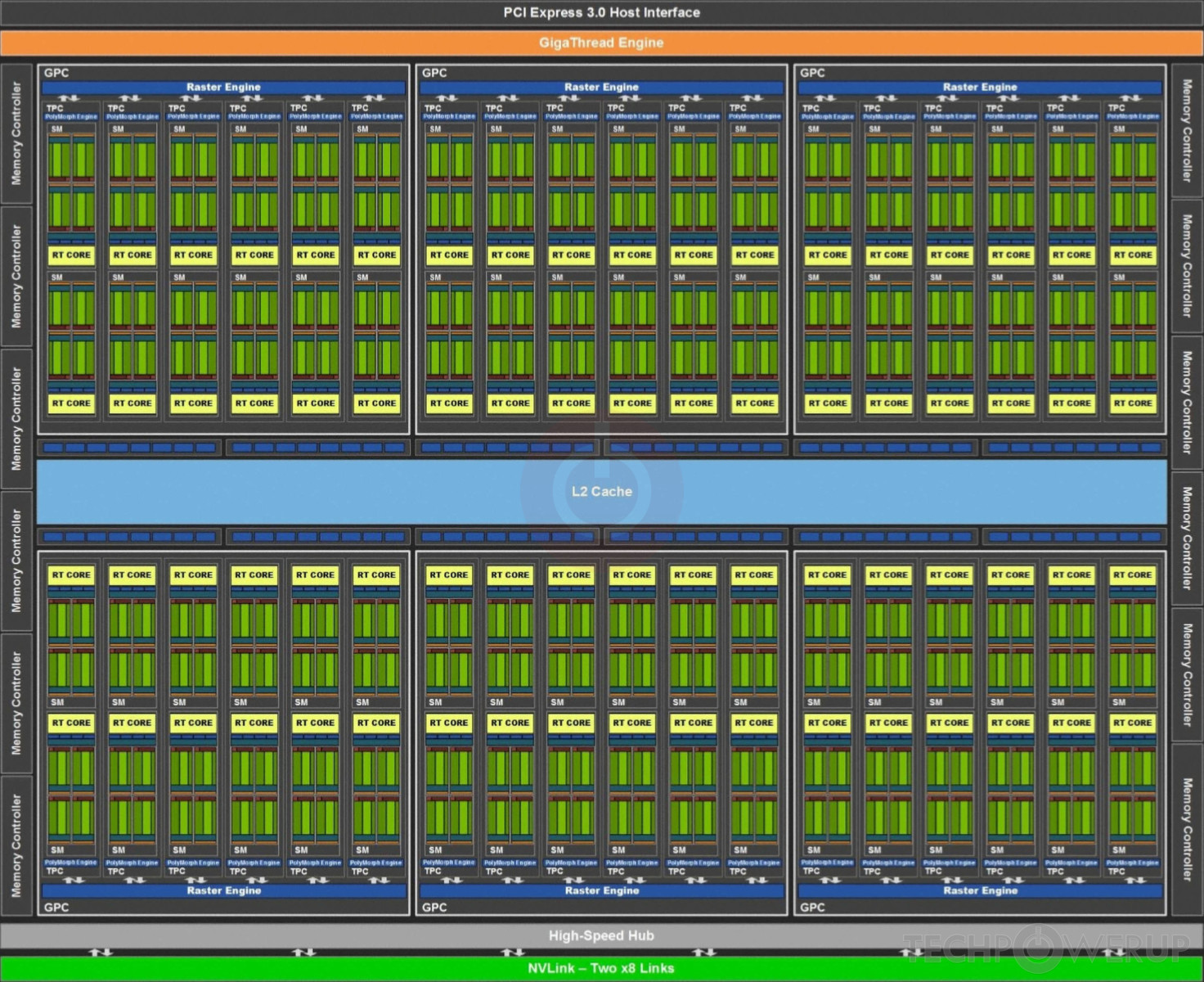
The streaming multiprocessors are the fundamental processing units of CUDA enabled GPUs. Each SM can execute hundreds of threads in parallel, and has all the resources needed to manage these threads.
Number of blocks and number of threads per block 
When the kernel is launched, each block of threads is sent to a single SM, and each SM can end up with multiple blocks to process.
The first conclusion we can draw is that if the number of blocks is lower than the number of SMs in the GPU, some of the SMs will be idle. That was the case in our first simple example above: we used 32 blocks, and we have 72 SMs on the Tesla T4. Therefore, 40 SMs remained unused.
To process a block, the SM partitions it into groups of 32 threads called warps . A warp executes one common instruction at a given time in parallel for all threads in the warp. So full efficiency is realized if all warps in the block are complete. Therefore, the number of threads per block needs to be a multiple of 32. Moreover, to limit latency, this number should not be too low.
Deciding which execution configuration to use is not easy, and the choice should be driven by performance analysis. However, here are some basic rules to get started:
- The number of blocks in the grid should be larger than the number of SMs on the GPU, typically 2 to 4 times larger.
- The number of threads per block should be a multiple of 32, typically between 128 and 512.
The Tesla T4 has 72 streaming multiprocessors. On paper, it will perform best on data arrays with a size larger than 72 2 128 ~ 20 000. And this is the bare minimum: this card will typically be used on arrays much larger than that. In our simple example above, we used an array of size 4096, which is way too small.
On the other hand, what if the data array is very large? Let's consider an array with one billion entries. Following the second rule above, we can choose a number of threads per block of 256, and we end up with 1e9 / 256 ~ 3 million blocks. Since the CUDA kernel launch overhead increases with the number of blocks, going for such a large number of blocks would hit performance. In the following, we will see how to use striding to solve this problem.
Striding 
This simple kernel deals with a single element of the input array:
@cuda.jit
def gpu_atan(x, out):
  idx = cuda.grid(1)
  out[idx] = math.atan(x[idx])
When the kernel is deployed, the GPU therefore needs to create as many threads as elements in the array, which potentially results in many blocks if the array is large.
On the contrary, a striding kernel deals with several elements of the input array, using a loop:
@cuda.jit
def gpu_atan_stride(x, out):
  start = cuda.grid(1)
  stride = cuda.gridsize(1)
  for i in range(start, x.shape[0], stride):
    out[i] = math.atan(x[i])
In this way, a given thread deals with several elements, and the number of threads is kept under control. Threads keep doing work in a coordinated way, and the GPU is not wasting time creating and scheduling threads.
Let's consider a small example with:
- an input data array of size 8
- blocks with 4 threads each
Without striding, we need to use two blocks so 8 threads in total, each dealing with a single element in the array:
a = np.arange(8, dtype=np.float32)
d_a = cuda.to_device(a)
d_out = cuda.device_array_like(d_a)

# 2 blocks of 4 threads
gpu_atan[2,4](d_a, d_out)
print(d_out.copy_to_host())
With striding, we can use a single block with 4 threads, in which case each thread deals with two elements. Specifically, in the code above:
-
startis the thread index, which is 0, 1, 2, 3 for the four threads, respectively. -
strideis the size of the grid, which is the total number of threads in the grid, here 4. -
x.shape[0]is the size of the input data arrayx, which is 8.
# 1 block of 4 threads
gpu_atan_stride[1,4](d_a, d_out)
print(d_out.copy_to_host())
Here are the elements processed by each thread:
for thread_index in range(4):
  print('thread', thread_index)
  for j in range(thread_index, 8, 4):
    print('\telement', j)
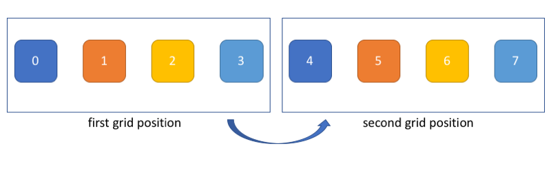
A useful way to think about this is to imagine that the grid is moving to process all elements in the input array, as shown below. In this picture, each color corresponds to a thread (e.g. thread 0 processes elements 0 and 4).
Of course, even though this representation can help you figure out how to code your striding, keep in mind that threads still proceed asynchronously. In other words, thread 0 might be done with elements 0 and 4 while thread 1 is still dealing with element 1.
Performance analysis 
In this section, we will study the influence of striding and of the execution configuration parameters in the processing of a large array.
So let's redefine our kernels (the simple one and the striding one:)
@cuda.jit
def gpu_atan(x, out):
  idx = cuda.grid(1)
  out[idx] = math.atan(x[idx])

@cuda.jit
def gpu_atan_stride(x, out):
  start = cuda.grid(1)
  stride = cuda.gridsize(1)
  for i in range(start, x.shape[0], stride):
    out[i] = math.atan(x[i])
Now we create a big array, we ship it to the device, and we create the output array on the device as usual:
import numpy as np
a = np.arange(256*1000000,dtype=np.float32)
# move input data to the device
d_a = cuda.to_device(a)
# create output data on the device
d_out = cuda.device_array_like(d_a)
First, let's see how fast we can process this array sequentially (in a single thread) on the GPU. We use the striding version here since, obviously, the simple version would only be able to process one element in a single thread.
# [1,1] means : 1 block with 1 thread
%time gpu_atan_stride[1, 1](d_a, d_out); cuda.synchronize()
Processing these 256 million values in a single thread on the GPU took almost a minute. Let's see how parallel processing can help us. For that, we choose an execution configuration by following our simple rules, and we use the non-striding kernel:
# RUN THIS TWICE.
# sometimes, the first time, the timing is way too large for some reason,
# and not representative of the actual timing
# you should get something around 13 ms.
%time gpu_atan[1000000,256](d_a, d_out); cuda.synchronize()
The parallel version is much faster as expected.
Now, let's try and see if the striding version brings any performance improvement:
# RUN THIS TWICE
%time gpu_atan_stride[50000,256](d_a, d_out); cuda.synchronize()
The gain is not very significant, you might have to rerun the two previous cells several times to convince yourself that there is indeed a gain. The amount of performance gain you'll get from striding will depend on the size of the input array, and on the work to be done by the kernel.
Exercise:
Try and change the number of blocks in the cell just above and re-run several times for each value to see how this parameter affects the timing. Try e.g. 100, 1 000, 100 000, and 500 000. Then, take the best value you could find for the number of blocks, and try to find the best value for the number of threads per block in the same way.
Multidimensional datasets : Matrix multiplication 
So far, we've been working with one-dimensional arrays, making use of a 1D grid of threads.
In the following 1D kernel,
cuda.grid(1)
returns a single index that identifies the position of the thread in the grid, and and
cuda.gridsize(1)
returns the length of the grid of threads:
@cuda.jit
def gpu_atan_stride(x, out):
  start = cuda.grid(1)
  stride = cuda.gridsize(1)
  for i in range(start, x.shape[0], stride):
    out[i] = math.atan(x[i])
As we will see, these functions also provide an easy interface for the processing of 2D and 3D data.
In this section, you will learn how to deploy a 2D grid of threads to process 2D data, and how to stride through 2D data. Then, you will implement a practical case: matrix multiplication.
A simple 2D kernel 
To learn the basic tools to work with 2D data, please consider the following kernel:
@cuda.jit
def gpu_2d(out):
  # get the thread coordinates in 2D
  i1, i2 = cuda.grid(2)
  out[i1][i2] = i1*10 + i2
As you can see, this kernel does not even have an input. Its goal is only to encode and record in the output 2D array the coordinates of the current thread.
Now, let's create the output data structure:
a = np.zeros(12).reshape(3,4)
a
We copy this data structure to the device, and we deploy the kernel, before fetching the results:
d_a = cuda.to_device(a)
# we use two blocks, side-by-side in the horizontal direction
blocks = (1,2)
# each block has 6 threads arranged in 3 lines and 2 columns
threads_per_block = (3,2)
gpu_2d[blocks, threads_per_block](d_a)
d_a.copy_to_host()
The first two columns were processed by the first block of threads, and the last two by the second block.
Looking at the kernel code and at the output above, we see that
i1
indexes the first dimension (the lines) while
i2
indexes the second dimension (the columns).
As in the 1D case, it's necessary to make sure that the grid covers the whole output data structure. For example, if we mess up in the description of the block structure, the last two columns remain unprocessed, and we actually access unallowed memory "below" our 2D array:
# need to send back the matrix of zeros
# to reset it on the device
d_a = cuda.to_device(a)
# here we mess up:
# we require two blocks on top of each other,
# and we get a grid with a total height of 2x3=6
# and a total width of 1x2=2...
gpu_2d[(2,1), (3,2)](d_a)
d_a.copy_to_host()
2D striding 
Striding in 2D is not much more difficult that in 1D. Again, let's take a very simple example, and first make sure that our implementation of striding is working:
@cuda.jit
def gpu_2d_stride(out):
  # get the thread coordinates in 2D
  s1, s2 = cuda.grid(2)
  # get the grid size in 2D
  d1, d2 = cuda.gridsize(2)
  for i1 in range(s1, out.shape[0], d1):
    for i2 in range(s2, out.shape[1], d2):
      out[i1][i2] = i1*10 + i2
We reset the output data on the device, and we deploy a
single
(3,2)
block. The grid therefore covers only half of the output array. But the striding will move the grid in the output array, making sure that the whole array is covered:
d_a = cuda.to_device(a)
gpu_2d_stride[(1,), (3,2)](d_a)
d_a.copy_to_host()
We get the same results as without striding. Now let's visualize striding with a slightly different kernel, which will register the starting point
(s1, s2)
of each thread:
@cuda.jit
def gpu_2d_start(out):
  # get the thread coordinates in 2D
  s1, s2 = cuda.grid(2)
  # get the grid size in 2D
  d1, d2 = cuda.gridsize(2)
  for i1 in range(s1, out.shape[0], d1):
    for i2 in range(s2, out.shape[1], d2):
      # note the difference w/r to the previous kernel
      out[i1][i2] = s1*10 + s2
d_a = cuda.to_device(a)
gpu_2d_start[(1,), (3,2)](d_a)
d_a.copy_to_host()
The elements with the same value are processed by the same thread, and we see that there is only one stride to the right.
Extending our 2D array, we see that striding occurs in both direction:
a = np.zeros(16).reshape(4,4)
d_a = cuda.to_device(a)
gpu_2d_start[(1,), (3,2)](d_a)
d_a.copy_to_host()
Here we have four strides arranged in a
(2,2)
structure. The strides at the bottom are incomplete, but the kernel is naturally protected against overflow since the loops are limited to the dimensions of the output array.
Exercise:
We see that thread
(0,0)
processes four elements of the output array just above. Look at the kernel code and find out in which order the thread processes these four elements.
2D matrix multiplication : theory 
Implement a 2D matrix multiplication kernel is an excellent way to confirm that we now master striding in 2D.
First, a little reminder. Two matrices A of size (m,n) and B of size (n,p) can be multiplied since the number of colums of matrix A is equal to the number of lines of matrix B. The product matrix C is then of size (m,p). And the value of one of the coefficients of matrix C is given by:
$$c_{ij} = \sum_{k=0}^{n} a_{ik} b_{kj}$$This might seem a bit complicated if you are new to linear algebra or haven't used it in a long time. So let's take a simple example in code. We create two matrices:
a = np.arange(6).reshape(2,3)
b = np.arange(12).reshape(3,4)
print(a)
print(b)
And we do the multiplication with numpy (on the CPU):
c = a.dot(b)
c
Matrix
a
is of size
(2,3)
and matrix
b
of size
(3,4)
, so the product matrix is of size
(2,4)
.
Let's consider for example the coefficient on the first line and second column of the product matrix, which is 23. This is c01. The summation equation above tells us that this coefficient is obtained by taking the coefficients of the first line of matrix a, and by multiplying them with the coefficients of the second column of matrix b, respectively, before summing everything.
We get:
c01 = a00*b01 + a01*b11 + a02*b21 = 0*1 + 1*5 + 2*9 = 23
A 2D matrix multiplication kernel 
As a first step, we will implement matrix multiplication without striding. So we will need one thread for each element in the output matrix. Here is the kernel:
@cuda.jit
def multiply(a, b, c):
  i1, i2 = cuda.grid(2)
  the_sum = 0
  for k in range(b.shape[0]): # or a.shape[1] since they are equal
    the_sum += a[i1][k]*b[k][i2]
  c[i1, i2] = the_sum
We ship the matrices
a
and
b
to the device, and create the output matrix
c
:
d_a = cuda.to_device(a)
d_b = cuda.to_device(b)
c = np.zeros((a.shape[0], b.shape[1]))
print(c.shape)
d_c = cuda.to_device(c)
Then, we deploy the kernel. We use a single block with 8 threads, arranged as a 2D array with 2 lines and 4 columns, matching the shape of the output matrix:
multiply[(1,), (2,4)](d_a, d_b, d_c)
print(d_c.copy_to_host())
Fine, we get the same results as with numpy.
Implementing striding is really no big deal. The only thing that could be a bit tricky is to remember that we need to stride on the output matrix, which has shape
(a.shape[0], b.shape[1])
. For striding, the inputs are irrelevant!
@cuda.jit
def multiply_stride(a, b, c):
  s1, s2 = cuda.grid(2)
  d1, d2 = cuda.gridsize(2)
  for i1 in range(s1, a.shape[0], d1):
    for i2 in range(s2, b.shape[1], d2):
      the_sum = 0
      for k in range(b.shape[0]): # or a.shape[1]
        the_sum += a[i1][k]*b[k][i2]
      c[i1, i2] = the_sum
# shipping back c to reset it on the device:
d_c = cuda.to_device(c)
# using a single block of shape (2,2)
# so we have 4 threads and each one produces
# two elements in the output matrix.
# in other words, the grid of (2,2) threads is moved
# once to the right in the output matrix.
multiply_stride[(1,), (2,2)](d_a, d_b, d_c)
print(d_c.copy_to_host())
What now?
In this post, you have learnt how to:
- use numba+CUDA on Google Colab;
- write your first custom CUDA kernels, to process 1D or 2D data.
For the sake of simplicity, I decided to show you how to implement relatively well-known and straightforward algorithms.
If you want to go further, you could try and implement the gaussian blur algorithm to smooth photos on the GPU. If you manage to do that, please feel free to post the input and output photograph in the comments. And if you don't, just ask questions, and I'll be happy to help!
Anyway, you should now be able to start implementing custom algorithms that can actually be useful to you.
But before you do that, I would advise you to first have a look at the libraries that are based on CUDA . What you need could already be there, and coded in a very efficient way by experts! For example, one could cite:
- cuDNN : GPU-accelerated library of primitives for deep neural networks. No need to code back-propagation or convolutional layers yourself!
- cuBLAS : GPU-accelerated linear algebra. hmm there was no need to spend so much time learning how to multiply matrices on the GPU...
- cuRAND : GPU-based random number generation
- cuFFT : Fast Fourier Transform
- ...
Please let me know what you think in the comments! I’ll try and answer all questions.
And if you liked this article, you can subscribe to my mailing list to be notified of new posts (no more than one mail per week I promise.)
Learn about Data Science and Machine Learning!
You can join my mailing list for new posts and exclusive content: